Models
Solid Mechanics Model / Solid Mechanics Model Cohesive
The solid mechanics model is a specific implementation of the Model interface dedicated to handle the equations of motion or
equations of equilibrium. The model is created for a given mesh. It will create
its own FEEngine object to compute the
interpolation, gradient, integration and assembly operations. A
SolidMechanicsModel object can simply
be created like this:
SolidMechanicsModel model(mesh);
where mesh is the mesh for which the equations are to be
solved. A second parameter called spatial_dimension can be
added after mesh if the spatial dimension of the problem is
different than that of the mesh.
This model contains at least the following six Arrays:
blocked_dofscontains a Boolean value for each degree of freedom specifying whether that degree is blocked or not. A Dirichlet boundary condition can be prescribed by setting the blocked_dofs value of a degree of freedom to
true. A Neumann boundary condition can be applied by setting the blocked_dofs value of a degree of freedom tofalse. The displacement, velocity and acceleration are computed for all degrees of freedom for which the blocked_dofs value is set tofalse. For the remaining degrees of freedom, the imposed values (zero by default after initialization) are kept.displacementcontains the displacements of all degrees of freedom. It can be either a computed displacement for free degrees of freedom or an imposed displacement in case of blocked ones (\(\vec{u}\) in the following).
velocitycontains the velocities of all degrees of freedom. As displacement, it contains computed or imposed velocities depending on the nature of the degrees of freedom (\(\dot{\vec{u}}\) in the following).
accelerationcontains the accelerations of all degrees of freedom. As displacement, it contains computed or imposed accelerations depending on the nature of the degrees of freedom (\(\ddot{\vec{u}}\) in the following).
external_forcecontains the external forces applied on the nodes (\(\vec{f}_{\st{ext}}\) in the following).
internal_forcecontains the internal forces on the nodes (\(\vec{f}_{\mathrm{int}}\) in the following).
Some examples to help to understand how to use this model will be
presented in the next sections. In addition to vector quantities, the solid
mechanics model can be queried for energies with the getEnergy which accepts an energy type as an
arguement (e.g. kinetic or potential).
Model Setup
Setting Initial Conditions
For a unique solution of the equations of motion, initial displacements and velocities for all degrees of freedom must be specified:
The solid mechanics model can be initialized as follows:
model.initFull()
This function initializes the internal arrays and sets them to zero. Initial displacements and velocities that are not equal to zero can be prescribed by running a loop over the total number of nodes. Here, the initial displacement in \(x\)-direction and the initial velocity in \(y\)-direction for all nodes is set to \(0.1\) and \(1\), respectively:
auto & disp = model.getDisplacement();
auto & velo = model.getVelocity();

for (Int node = 0; node < mesh.getNbNodes(); ++node) {
    disp(node, 0) = 0.1;
    velo(node, 1) = 1.;
}
Setting Boundary Conditions
This section explains how to impose Dirichlet or Neumann boundary conditions. A Dirichlet boundary condition specifies the values that the displacement needs to take for every point \(x\) at the boundary (\(\Gamma_u\)) of the problem domain (Fig. 6):
A Neumann boundary condition imposes the value of the gradient of the solution at the boundary \(\Gamma_t\) of the problem domain (Fig. 6):

Fig. 6 Problem domain \(\Omega\) with boundary in three dimensions. The Dirchelet and the Neumann regions of the boundary are denoted with \(\Gamma_u\) and \(\Gamma_t\), respecitvely.
Different ways of imposing these boundary conditions exist. A basic way is to loop over nodes or elements at the boundary and apply local values. A more advanced method consists of using the notion of the boundary of the mesh. In the following both ways are presented.
Starting with the basic approach, as mentioned, the Dirichlet boundary
conditions can be applied by looping over the nodes and assigning the
required values. Fig. 7 shows a beam with a
fixed support on the left side. On the right end of the beam, a load
is applied. At the fixed support, the displacement has a given
value. For this example, the displacements in both the \(x\) and the
\(y\)-direction are set to zero. Implementing this displacement boundary
condition is similar to the implementation of initial displacement
conditions described above. However, in order to impose a displacement
boundary condition for all time steps, the corresponding nodes need to
be marked as boundary nodes using the function blocked. While,
in order to impose a load on the right side, the nodes are not marked.
The detail codes are shown as follows
auto & blocked = model.getBlockedDOFs();
const auto & pos = mesh.getNodes();

UInt nb_nodes = mesh.getNbNodes();

for (Int node = 0; node < nb_nodes; ++node) {
  if(Math::are_float_equal(pos(node, _x), 0)) {
    blocked(node, _x) = true; // block dof in x-direction
    blocked(node, _y) = true; // block dof in y-direction
    disp(node, _x) = 0.; // fixed displacement in x-direction
    disp(node, _y) = 0.; // fixed displacement in y-direction
  } else if (Math::are_float_equal(pos(node, _y), 0)) {
    blocked(node, _x) = false; // unblock dof in x-direction
    forces(node, _x) = 10.;    // force in x-direction
  }
}

Fig. 7 Beam with fixed support and load.
For the more advanced approach, one needs the notion of a boundary in
the mesh. Therefore, the boundary should be created before boundary
condition functors can be applied. Generally the boundary can be
specified from the mesh file or the geometry. For the first case, the
function createGroupsFromMeshData is called. This function
can read any types of mesh data which are provided in the mesh
file. If the mesh file is created with Gmsh, the function takes one
input strings which is either tag_0, tag_1 or
physical_names. The first two tags are assigned by Gmsh to
each element which shows the physical group that they belong to. In
Gmsh, it is also possible to consider strings for different groups of
elements. These elements can be separated by giving a string
physical_names to the function
createGroupsFromMeshData
mesh.createGroupsFromMeshData<std::string>("physical_names").
Boundary conditions support can also be created from the geometry by calling
createBoundaryGroupFromGeometry. This function gathers all the elements on
the boundary of the geometry.
To apply the required boundary conditions, the function applyBC needs to be called on a
SolidMechanicsModel. This function
gets a Dirichlet or Neumann functor and a string which specifies the desired
boundary on which the boundary conditions is to be applied. The functors specify
the type of conditions to apply. Three built-in functors for Dirichlet exist:
FlagOnly, FixedValue and IncrementValue. The functor FlagOnly is used if a
point is fixed in a given direction. Therefore, the input parameter to this
functor is only the fixed direction. The FixedValue functor is used when a
displacement value is applied in a fixed direction. The IncrementValue
applies an increment to the displacement in a given direction. The following
code shows the utilization of three functors for the top, bottom and side
surface of the mesh which were already defined in the Gmsh
model.applyBC(BC::Dirichlet::FixedValue(13.0, _y), "Top");
model.applyBC(BC::Dirichlet::FlagOnly(_x), "Bottom");
model.applyBC(BC::Dirichlet::IncrementValue(13.0, _x), "Side");
To apply a Neumann boundary condition, the applied traction or stress should be
specified before. In case of specifying the traction on the surface, the functor
FromTraction of Neumann
boundary conditions is called. Otherwise, the functor FromStress should be called which gets the stress tensor
as an input parameter
Vector<Real> surface_traction{0., 0., 1.};
auto surface_stress(3, 3) = Matrix<Real>::eye(3);

model.applyBC(BC::Neumann::FromTraction(surface_traction), "Bottom");
model.applyBC(BC::Neumann::FromStress(surface_stress), "Top");
If the boundary conditions need to be removed during the simulation, a functor is called from the Neumann boundary condition to free those boundary conditions from the desired boundary
model.applyBC(BC::Neumann::FreeBoundary(), "Side");
User specified functors can also be implemented. A full example for
setting both initial and boundary conditions can be found in
examples/boundary_conditions.cc. The problem solved
in this example is shown in Fig. 8. It consists
of a plate that is fixed with movable supports on the left and bottom
side. On the right side, a traction, which increases linearly with the
number of time steps, is applied. The initial displacement and
velocity in \(x\)-direction at all free nodes is zero and two
respectively.

Fig. 8 Plate on movable supports.
As it is mentioned in Section Mesh, node and element groups can be used to assign the boundary conditions. A generic example is given below with a Dirichlet boundary condition:
// create a node group
NodeGroup & node_group = mesh.createNodeGroup("nodes_fix");

/* fill the node group with the nodes you want */

// create an element group using the existing node group
mesh.createElementGroupFromNodeGroup("el_fix",
                                     "nodes_fix",
                                     spatial_dimension-1);

// boundary condition can be applied using the element group name
model.applyBC(BC::Dirichlet::FixedValue(0.0, _x), "el_fix");
Material Selector
If the user wants to assign different materials to different
finite elements groups in Akantu, a material selector has to be
used. By default, Akantu assigns the first valid material in the
material file to all elements present in the model (regular continuum
materials are assigned to the regular elements and cohesive materials
are assigned to cohesive elements or element facets).
To assign different materials to specific elements, mesh data information such
as tag information or specified physical names can be used.
MeshDataMaterialSelector class
uses this information to assign different materials. With the proper physical
name or tag name and index, different materials can be assigned as demonstrated
in the examples below:
auto mat_selector =
   std::make_shared<MeshDataMaterialSelector<std::string>>("physical_names",
                                                           model);
model.setMaterialSelector(mat_selector);
In this example the physical names specified in a GMSH geometry file will by used to match the material names in the input file.
Another example would be to use the first (tag_0) or the second
(tag_1) tag associated to each elements in the mesh:
auto mat_selector = std::make_shared<MeshDataMaterialSelector<UInt>>(
    "tag_1", model, first_index);
model.setMaterialSelector(*mat_selector);
where first_index (default is 1) is the value of tag_1 that will
be associated to the first material in the material input file. The following
values of the tag will be associated with the following materials.
There are four different material selectors pre-defined in Akantu.
MaterialSelector and
DefaultMaterialSelector is used
to assign a material to regular elements by default. For the regular elements,
as in the example above, MeshDataMaterialSelector can be used to assign different materials to
different elements.
Apart from the Akantu’s default material selectors, users can always
develop their own classes in the main code to tackle various
multi-material assignment situations.
For cohesive material, Akantu has a pre-defined material selector to assign
the first cohesive material by default to the cohesive elements which is called
DefaultMaterialCohesiveSelector and it inherits its properties from
DefaultMaterialSelector. Multiple
cohesive materials can be assigned using mesh data information (for more
details, see Intrinsic approach).
Insertion of Cohesive Elements
Cohesive elements are currently compatible only with static simulation and dynamic simulation with an explicit time integration scheme (see section Explicit Time Integration). They do not have to be inserted when the mesh is generated (intrinsic) but can be added during the simulation (extrinsic). At any time during the simulation, it is possible to access the following energies with the relative function:
Real Ed = model.getEnergy("dissipated");
Real Er = model.getEnergy("reversible");
Real Ec = model.getEnergy("contact");
A new model have to be call in a very similar way that the solid mechanics model:
SolidMechanicsModelCohesive model(mesh);
model.initFull(_analysis_method = _explicit_lumped_mass,
               _is_extrinsic = true);
Cohesive element insertion can be either realized at the beginning of
the simulation or it can be carried out dynamically during the
simulation. The first approach is called intrinsic, the second
one extrinsic. When an element is present from the beginning, a
bi-linear or exponential cohesive law should be used instead of a
linear one. A bi-linear law works exactly like a linear one except for
an additional parameter \(\delta_0\) separating an initial linear
elastic part from the linear irreversible one. For additional details
concerning cohesive laws see Cohesive Constitutive laws.

Fig. 9 Insertion of a cohesive element.
Extrinsic cohesive elements are dynamically inserted between two standard elements when
in which \(\sigma_\st{n}\) is the tensile normal traction and $tau$ the resulting tangential one (Fig. 9).
Extrinsic approach
During the simulation, stress has to be checked along each facet in order to
insert cohesive elements where the stress criterion is reached. This check is
performed by calling the method checkCohesiveStress, as example before
each step resolution:
model.checkCohesiveStress();
model.solveStep();
The area where stresses are checked and cohesive elements inserted can be
limited using the method setLimit on the CohesiveInserter during initialization. As example, to limit
insertion in the range \([-1.5, 1.5]\) in the $x$ direction:
auto & inserter = model.getElementInserter();
inserter.setLimit(_x, -1.5, 1.5);
Additional restrictions with respect to \(_y\) and \(_z\) directions can be added as well.
Intrinsic approach
Intrinsic cohesive elements are inserted in the mesh with the method
initFull.
Similarly, the range of insertion can be limited with setLimit before the initFull call.
In both cases extrinsic and intrinsic the insertion can be restricted to surfaces or element groups. To do so the list of groups should be specified in the input file.
model solid_mechanics_model_cohesive [
  cohesive_inserter [
    cohesive_surfaces = [surface1, surface2, ...]
    cohesive_zones = [group1, group2, ...]
  ]

  material cohesive_linear [
    name = insertion
    beta = 1
    G_c = 10
    sigma_c = 1e6
  ]
]
cohesive_surfaces defines are the physical surfaces defined in the mesh
(Curves in 1D and Surfaces in 2D) on which the insertion is allowed,
cohesive_zones are the physical volumes in which the insertion is allowed
(Surfaces in 2D and Volumes in 3D).
Static Analysis
The SolidMechanicsModel class can
handle different analysis methods, the first one being presented is the static
case. In this case, the equation to solve is
where \(\mat{K}\) is the global stiffness matrix, \(\vec{u}\) the displacement vector and \(\vec{f}_\st{ext}\) the vector of external forces applied to the system.
To solve such a problem, the static solver of the
SolidMechanicsModel object is used.
First, a model has to be created and initialized. To create the model, a mesh
(which can be read from a file) is needed, as explained in
sect-common-mesh. Once an instance of a
SolidMechanicsModel is obtained, the
easiest way to initialize it is to use the initFull method by giving the
SolidMechanicsModelOptions.
These options specify the type of analysis to be performed and whether the
materials should be initialized with initMaterials or not
SolidMechanicsModel model(mesh);
model.initFull(_analysis_method = _static);
Here, a static analysis is chosen by passing the argument
_static to the method. By default, the
Boolean for no initialization of the materials is set to false, so that they are
initialized during the initFull. The method initFull also initializes
all appropriate vectors to zero.
Note
The solver type and its parameters can also be configured directly in the input file. See Model solver configuration for the full syntax.
Once the model is created and initialized, the
boundary conditions can be set as explained in Section Setting Boundary Conditions.
Boundary conditions will prescribe the external forces for some free degrees of
freedom \(\vec{f}_\st{ext}\) and displacements for some others. At this
point of the analysis, the function
solveStep can be called
auto & solver = model.getNonLinearSolver();
solver.set("max_iterations", 1);
solver.set("threshold", 1e-4);
solver.set("convergence_type", SolveConvergenceCriteria::_residual);

model.solveStep();
This function is templated by the solving method and the convergence criterion and takes two arguments: the tolerance and the maximum number of iterations (100 by default), which are \(10^{-4}\) and \(1\) for this example. The modified Newton-Raphson method is chosen to solve the system. In this method, the equilibrium equation (Eq. 1) is modified in order to apply a Newton-Raphson convergence algorithm:
where \(\delta\vec{u}\) is the increment of displacement to be added from
one iteration to the other, and \(i\) is the Newton-Raphson iteration
counter. By invoking the solveStep method in the first step, the global
stiffness matrix \(\mat{K}\) from (Eq. 1) is automatically
assembled. A Newton-Raphson iteration is subsequently started, \(\mat{K}\)
is updated according to the displacement computed at the previous iteration and
one loops until the forces are balanced
(SolveConvergenceCriteria::_residual), i.e. \(||\vec{r}|| <\)
threshold. One can also
iterate until the increment of displacement is zero
(SolveConvergenceCriteria::_solution) which also means that the
equilibrium is found. For a linear elastic problem, the solution is obtained in
one iteration and therefore the maximum number of iterations can be set to one.
But for a non-linear case, one needs to iterate as long as the norm of the
residual exceeds the tolerance threshold and therefore the maximum number of
iterations has to be higher, e.g. \(100\)
solver.set("max_iterations", 100);
model.solveStep();
At the end of the analysis, the final solution is stored in the
displacement vector. A full example of how to solve a static
problem is presented in the code examples/static/static.cc.
This example is composed of a 2D plate of steel, blocked with rollers
on the left and bottom sides as shown in Fig. 10.
The nodes from the right side of the sample are displaced by \(0.01\%\)
of the length of the plate.

Fig. 10 Numerical setup.
The results of this analysis is depicted in Fig. 11.
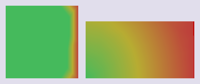
Fig. 11 Solution of the static analysis. Left: the initial condition, right: the solution (deformation magnified 50 times).
Dynamic Methods
Different ways to solve the equations of motion are implemented in the solid mechanics model. The complete equations that should be solved are:
where \(\mat{M}\), \(\mat{C}\) and \(\mat{K}\) are the mass, damping and stiffness matrices, respectively.
In the previous section, it has already been discussed how to solve this
equation in the static case, where \(\ddot{\vec{u}} = \dot{\vec{u}} = 0\).
Here the method to solve this equation in the general case will be presented.
For this purpose, a time discretization has to be specified. The most common
discretization method in solid mechanics is the Newmark-\(\beta\) method,
which is also the default in Akantu.
For the Newmark-\(\beta\) method, (Eq. 2) becomes a system of three equations (see [Cur92, HB83] for more details):
In these new equations, \(\ddot{\vec{u}}_{n}\), \(\dot{\vec{u}}_{n}\) and \(\vec{u}_{n}\) are the approximations of \(\ddot{\vec{u}}(t_n)\), \(\dot{\vec{u}}(t_n)\) and \(\vec{u}(t_n)\). Eq. 3 is the equation of motion discretized in space (finite-element discretization), and the equations above are discretized in both space and time (Newmark discretization). The \(\alpha\) and \(\beta\) parameters determine the stability and the accuracy of the algorithm. Classical values for \(\alpha\) and \(\beta\) are usually \(\beta = 1/2\) for no numerical damping and \(0 < \alpha < 1/2\).
\(alpha\) |
Method (\(beta = 1/2\)) |
Type |
|---|---|---|
\(0\) |
central difference |
explicit |
\(\frac{1}{6}\) |
Fox-Goodwin(royal road) |
implicit |
\(\frac{1}{3}\) |
Linear acceleration |
implicit |
\(\frac{1}{2}\) |
Average acceleration (trapeziodal rule) |
implicit |
The solution of this system of equations, (Eq. 3) is split into a predictor and a corrector system of equations. Moreover, in the case of a non-linear equations, an iterative algorithm such as the Newton-Raphson method is applied. The system of equations can be written as:
Predictor:
\[\begin{split}\vec{u}_{n+1}^{0} &= \vec{u}_{n} + \Delta t \dot{\vec{u}}_{n} + \frac{\Delta t^2}{2} \ddot{\vec{u}}_{n} \\ \dot{\vec{u}}_{n+1}^{0} &= \dot{\vec{u}}_{n} + \Delta t \ddot{\vec{u}}_{n} \\ \ddot{\vec{u}}_{n+1}^{0} &= \ddot{\vec{u}}_{n}\end{split}\]Solve:
\[\begin{split}\left(c \mat{M} + d \mat{C} + e \mat{K}_{n+1}^i\right) \vec{w} &= {\vec{f}_{\st{ext}}}_{\,n+1} - {\vec{f}_{\st{int}}}_{\,n+1}^i - \mat{C} \dot{\vec{u}}_{n+1}^i - \mat{M} \ddot{\vec{u}}_{n+1}^i\\ &= \vec{r}_{n+1}^i\end{split}\]Corrector:
\[\begin{split}\ddot{\vec{u}}_{n+1}^{i+1} &= \ddot{\vec{u}}_{n+1}^{i} +c \vec{w} \\ \dot{\vec{u}}_{n+1}^{i+1} &= \dot{\vec{u}}_{n+1}^{i} + d\vec{w} \\ \vec{u}_{n+1}^{i+1} &= \vec{u}_{n+1}^{i} + e \vec{w}\end{split}\]
where \(i\) is the Newton-Raphson iteration counter and \(c\), \(d\) and \(e\) are parameters depending on the method used to solve the equations
\(vec{w}\) |
\(e\) |
\(d\) |
\(c\) |
|
|---|---|---|---|---|
in acceleration |
\(\delta\ddot{\vec{u}}\) |
\(\alpha\beta\Delta t^2\) |
\(\beta\Delta t\) |
\(1\) |
in velocity |
\(\delta\dot{\vec{u}}\) |
\(\alpha\Delta t\) |
\(1\) |
\(\frac{1}{\beta\Delta t}\) |
in displacement |
\(\delta\vec{u}\) |
\(1\) |
\(\frac{1}{\alpha\Delta t}\) |
\(\frac{1}{\alpha\beta \Delta t^2}\) |
Note
If you want to use the implicit solver Akantu should be compiled at
least with one sparse matrix solver such as Mumps [spa].
Implicit Time Integration
To solve a problem with an implicit time integration scheme, first a
SolidMechanicsModel object has to be
created and initialized. Then the initial and boundary conditions have to be
set. Everything is similar to the example in the static case
(Static Analysis), however, in this case the implicit dynamic
scheme is selected at the initialization of the model:
SolidMechanicsModel model(mesh);
model.initFull(_analysis_method = _implicit_dynamic);
Because a dynamic simulation is conducted, an integration time step
\(\Delta t\) has to be specified. In the case of implicit simulations,
Akantu implements a trapezoidal rule by default. That is to say
\(\alpha = 1/2\) and \(\beta = 1/2\) which is unconditionally
stable. Therefore the value of the time step can be chosen arbitrarily
within reason:
model.setTimeStep(time_step);
Since the system has to be solved for a given amount of time steps, the
method solveStep(), (which has already been used in the static
example in Static Analysis), is called inside a time
loop:
/// time loop
Real time = 0.;

auto & solver = model.getNonLinearSolver();
solver.set("max_iterations", 100);
solver.set("threshold", 1e-12);
solver.set("convergence_type", SolveConvergenceCriteria::_solution);

for (Int s = 1; time <max_time; ++s, time += time_step) {
    model.solveStep();
}
An example of solid mechanics with an implicit time integration scheme is
presented in examples/implicit/implicit_dynamic.cc. This example consists of
a 3D beam of
\(10\mathrm{m}\times1\mathrm{m}\times1\mathrm{m}\) blocked
on one side and is on a roller on the other side. A constant force of
\(5\mathrm{kN}\) is applied in its middle.
Fig. 12 presents the geometry of this case. The
material used is a fictitious linear elastic material with a density of
\(1000 \mathrm{kg/m}^3\), a Young’s Modulus of
\(120 \mathrm{MPa}\) and Poisson’s ratio of \(0.3\). These values
were chosen to simplify the analytical solution.
An approximation of the dynamic response of the middle point of the beam is given by:

Fig. 12 Numerical setup.
Fig. 13 presents the deformed beam at 3 different times during the simulation: time steps 0, 1000 and 2000.
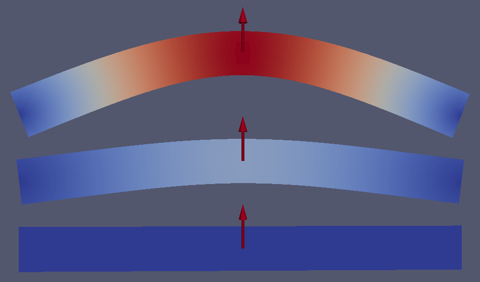
Fig. 13 Deformed beam at three different times (displacement \(\times 10\)).
Explicit Time Integration
The explicit dynamic time integration scheme is based on the
Newmark-\(\beta\) scheme with \(\alpha=0\) (see equations
Eq. 3-eqn-finite-difference-2). In
Akantu, \(\beta\) is defaults to \(\beta=1/2\), see section
Dynamic Methods.
The initialization of the simulation is similar to the static and implicit
dynamic version. The model is created from the SolidMechanicsModel class. In the initialization, the explicit scheme
is selected using the _explicit_lumped_mass constant:
SolidMechanicsModel model(mesh);
model.initFull(_analysis_method = _explicit_lumped_mass);
Note
Writing model.initFull() or model.initFull(); is
equivalent to use the _explicit_lumped_mass keyword, as this
is the default case.
The explicit time integration scheme implemented in Akantu uses a
lumped mass matrix \(\mat{M}\) (reducing the computational cost). This
matrix is assembled by distributing the mass of each element onto its
nodes. The resulting \(\mat{M}\) is therefore a diagonal matrix stored
in the mass vector of the model.
The explicit integration scheme is conditionally stable. The time step has to be smaller than the stable time step which is obtained in Akantu as follows:
critical_time_step = model.getStableTimeStep();
The stable time step corresponds to the time the fastest wave (the compressive wave) needs to travel the characteristic length of the mesh:
where \(\Delta x\) is a characteristic length (eg the inradius in the case of linear triangle element) and \(c\) is the celerity of the fastest wave in the material. It is generally the compressive wave of celerity \(c = \sqrt{\frac{2 \mu + \lambda}{\rho}}\), \(\mu\) and \(\lambda\) are the first and second Lame’s coefficients and \(\rho\) is the density. However, it is recommended to impose a time step that is smaller than the stable time step, for instance, by multiplying the stable time step by a safety factor smaller than one:
const Real safety_time_factor = 0.8;
Real applied_time_step = critical_time_step * safety_time_factor;
model.setTimeStep(applied_time_step);
The initial displacement and velocity fields are, by default, equal to zero if not given specifically by the user (see Setting Initial Conditions).
Like in implicit dynamics, a time loop is used in which the
displacement, velocity and acceleration fields are updated at each
time step. The values of these fields are obtained from the
Newmark-\(\beta\) equations with \(\beta=1/2\) and \(\alpha=0\). In Akantu
these computations at each time step are invoked by calling the
function solveStep:
for (Int s = 1; (s-1)*applied_time_step < total_time; ++s) {
  model.solveStep();
}
The method solveStep wraps the four following functions:
model.explicitPred()allows to compute the displacement field at \(t+1\) and a part of the velocity field at \(t+1\), denoted by \(\vec{\dot{u}^{\st{p}}}_{n+1}\), which will be used later in the methodmodel.explicitCorr(). The equations are:\[\begin{split}\vec{u}_{n+1} &= \vec{u}_{n} + \Delta t \vec{\dot{u}}_{n} + \frac{\Delta t^2}{2} \vec{\ddot{u}}_{n}\\ \vec{\dot{u}^{\st{p}}}_{n+1} &= \vec{\dot{u}}_{n} + \Delta t \vec{\ddot{u}}_{n}\end{split}\]model.updateResidual()andmodel.updateAcceleration()compute the acceleration increment \(\delta \vec{\ddot{u}}\):\[\left(\mat{M} + \frac{1}{2} \Delta t \mat{C}\right) \delta \vec{\ddot{u}} = \vec{f_{\st{ext}}} - \vec{f}_{\st{int}\, n+1} - \mat{C} \vec{\dot{u}^{\st{p}}}_{n+1} - \mat{M} \vec{\ddot{u}}_{n}\]- The internal force \(\vec{f}_{\st{int}\, n+1}\) is computed from the
displacement \(\vec{u}_{n+1}\) based on the constitutive law.
model.explicitCorr()computes the velocity and acceleration fields at \(t+1\):\[\begin{split}\vec{\dot{u}}_{n+1} &= \vec{\dot{u}^{\st{p}}}_{n+1} + \frac{\Delta t}{2} \delta \vec{\ddot{u}} \\ \vec{\ddot{u}}_{n+1} &= \vec{\ddot{u}}_{n} + \delta \vec{\ddot{u}}\end{split}\]
The use of an explicit time integration scheme is illustrated by the example:
examples/explicit/explicit_dynamic.cc. This example models the propagation
of a wave in a steel beam. The beam and the applied displacement in the
\(x\) direction are shown in Fig. 14.

Fig. 14 Numerical setup.
The length and height of the beam are \(L={10}\textrm{m}\) and \(h = {1}\textrm{m}\), respectively. The material is linear elastic, homogeneous and isotropic (density: \(7800\mathrm{kg/m}^3\), Young’s modulus: \(210\mathrm{GPa}\) and Poisson’s ratio: \(0.3\)). The imposed displacement follow a Gaussian function with a maximum amplitude of \(A = {0.01}\textrm{m}\). The potential, kinetic and total energies are computed. The safety factor is equal to \(0.8\).
Constitutive Laws
In order to compute an element’s response to deformation, one needs to use an appropriate constitutive relationship. The constitutive law is used to compute the element’s stresses from the element’s strains.
In the finite-element discretization, the constitutive formulation is applied to every quadrature point of each element. When the implicit formulation is used, the tangent matrix has to be computed.
element_material vector. For
every material assigned to the problem one has to specify the material
characteristics (constitutive behavior and material properties) using
the text input file (see Material section).Akantu provides a special data structure, the at InternalField. The internal fields are inheriting from the at
ElementTypeMapArray. Furthermore,
it provides several functions for initialization, auto-resizing and auto
removal of quadrature points.The constitutive law is precised within an input file. The dedicated material section
is then read by initFull
method of SolidMechanicsModel which
initializes the different materials specified with the following convention
material constitutive_law [
  name = value
  rho = value
  ...
]
where constitutive_law is the adopted constitutive law, followed by
the material properties listed one by line in the bracket (e.g.,
name and density \(rho\). Some constitutive laws can also
have an optional flavor.
For certain materials, it is possible to activate the large deformation strain and stress evaluations. Internally the strain measure becomes the right Cauchy–Green deformation tensor and the evaluated stress measure becomes the Piola-Kirchhoff stress tensor. This is activated by using:
material constitutive_law [
  finite_deformation = true # Activates the large deformation routines (bool)
  ...
]
Sometimes it is also desired to generate random distributions of internal parameters. An example might be the critical stress at which the material fails. To generate such a field, in the text input file, a random quantity needs be added to the base value:
All parameters are real numbers. For the uniform distribution, minimum and maximum values have to be specified. Random parameters are defined as a \(base\) value to which we add a random number that follows the chosen distribution.
The Uniform distribution is gives a random values between in \([min, max)\). The Weibull distribution is characterized by the following cumulative distribution function:
which depends on \(m\) and \(\lambda\), which are the shape parameter and the scale parameter. These random distributions are different each time the code is executed. In order to obtain always the same one, it possible to manually set the seed that is the number from which these pseudo-random distributions are created. This can be done by adding the following line to the input file outside the material parameters environments:
seed = 1.0
where the value 1.0 can be substituted with any number. Currently
Akantu can reproduce always the same distribution when the seed is
specified only in serial. The value of the seed can be also
specified directly in the code (for instance in the main file) with the
command:
RandGenerator<Real>::seed(1.0)
The same command, with empty brackets, can be used to check the value of the seed used in the simulation.
The following sections describe the constitutive models implemented in
Akantu.
Elastic
The elastic law is a commonly used constitutive relationship that can be used for a wide range of engineering materials (e.g., metals, concrete, rock, wood, glass, rubber, etc.) provided that the strains remain small (i.e., small deformation and stress lower than yield strength).
The elastic laws are often expressed as \(\boldsymbol{\sigma} = \boldsymbol{C}:\boldsymbol{\varepsilon}\) with where \(\boldsymbol{\sigma}\) is the Cauchy stress tensor, \(\boldsymbol{\varepsilon}\) represents the infinitesimal strain tensor and \(\boldsymbol{C}\) is the elastic modulus tensor.
Linear isotropic
Keyword: elastic
Material description with input file:
#input.dat

material elastic [
  name = steel
  rho = 7800                  # density (Real)
  E   = 2.1e11                # young's modulus (Real)
  nu  = 0.3                   # poisson's ratio (Real)
  Plane_stress = false        # Plane stress simplification (only 2D problems) (bool)
  finite_deformation = false  # activates the evaluation of strains with green's tensor (bool)
]
Available energies Energies:
potential: elastic potential energy
The linear isotropic elastic behavior is described by Hooke’s law, which states that the stress is linearly proportional to the applied strain (material behaves like an ideal spring), as illustrated in Fig. 15.

Fig. 15 Stress-strain curve of elastic material and schematic representation of Hooke’s law, denoted as a spring.
The equation that relates the strains to the displacements is: point) from the displacements as follows:
where \(\boldsymbol{\varepsilon}\) represents the infinitesimal strain tensor, \(\nabla_{0}\boldsymbol{u}\) the displacement gradient tensor according to the initial configuration. The constitutive equation for isotropic homogeneous media can be expressed as:
where \(\boldsymbol{\sigma}\) is the Cauchy stress tensor (\(\lambda\) and \(\mu\) are the the first and second Lame’s coefficients).
In Voigt notation this correspond to
This formulation is not sufficient to represent all elastic material behavior. Some materials have characteristic orientation that have to be taken into account. To represent this anisotropy a more general stress-strain law has to be used, as shown below.
Linear anisotropic
Keyword: elastic_anisotropic
Material description with input file:
#input.dat

material elastic_anisotropic [
  name = aluminum
  rho = 1.6465129043044597 # density (Real)

  C11 = 105.092023         # Coefficient ij of material tensor C (Real)
  C12 = 59.4637759         # all the 36 values
  C13 = 59.4637759         # in Voigt notation can be entered
  C14 = 0                  # zero coefficients can be omited
  C15 = 0
  C16 = 0
  C22 = 105.092023
  C23 = 59.4637759
  C24 = 0
  C25 = 0
  C26 = 0
  C33 = 105.092023
  C34 = 0
  C35 = 0
  C36 = 0
  C44 = 30.6596356
  C45 = 0
  C46 = 0
  C55 = 30.6596356
  C56 = 0
  C66 = 30.6596356

  n1 = [-1, 1,  0]         # Direction of first material axis  (Vector<Real>)
  n2 = [ 1, 1,  1]         # Direction of second material axis (Vector<Real>)
  n3 = [ 1, 1, -2]         # Direction of thrid material axis  (Vector<Real>)
]
We define the elastic modulus tensor as follows:
To simplify the writing of input files the \(\boldsymbol{C}\) tensor is expressed in the material basis. And this basis as to be given too. This basis \(\Omega_{{\mathrm{mat}}} = \{\boldsymbol{n_1}, \boldsymbol{n_2}, \boldsymbol{n_3}\}\) is used to define the rotation \(R_{ij} = \boldsymbol{n_j} . \boldsymbol{e_i}\). And \(\boldsymbol{C}\) can be rotated in the global basis \(\Omega = \{\boldsymbol{e_1}, \boldsymbol{e_2}, \boldsymbol{e_3}\}\) as follow:
Linear orthotropic
Keyword: elastic_orthotropic
Inherits from elastic_anisotropic
Material description with input file:
#input.dat

material elastic_orthotropic [
  name = test_mat_1
  rho  = 1           # density

  n1 = [-1, 1,  0]   # Direction of first material axis  (Vector<Real>)
  n2 = [ 1, 1,  1]   # Direction of second material axis (Vector<Real>)
  n3 = [ 1, 1, -2]   # Direction of thrid material axis  (Vector<Real>)

  E1 = 1             # Young's modulus in direction n1 (Real)
  E2 = 2             # Young's modulus in direction n2 (Real)
  E3 = 3             # Young's modulus in direction n3 (Real)
  nu12 = 0.1          # Poisson's ratio 12 (Real)
  nu13 = 0.2          # Poisson's ratio 13 (Real)
  nu23 = 0.3          # Poisson's ratio 23 (Real)

  G12 = 0.5          # Shear modulus 12 (Real)
  G13 = 1            # Shear modulus 13 (Real)
  G23 = 2            # Shear modulus 23 (Real)
]
A particular case of anisotropy is when the material basis is orthogonal in which case the elastic modulus tensor can be simplified and rewritten in terms of 9 independents material parameters.
The Poisson ratios follow the rule \(\nu_{ij} = \nu_{ji} E_i / E_j\).
Neo-Hookean
Keyword: neohookean
Inherits from elastic
Material description with input file:
#input.dat

material neohookean [
  name = material_name
  rho = 7800                  # density (Real)
  E   = 2.1e11                # young's modulus (Real)
  nu  = 0.3                   # poisson's ratio (Real)
]
The hyperelastic Neo-Hookean constitutive law results from an extension of the linear elastic relationship (Hooke’s Law) for large deformation. Thus, the model predicts nonlinear stress-strain behavior for bodies undergoing large deformations.

Fig. 16 Neo-hookean Stress-strain curve.
As illustrated in Fig. 16, the behavior is initially linear and the mechanical behavior is very close to the corresponding linear elastic material. This constitutive relationship, which accounts for compressibility, is a modified version of the one proposed by Ronald Rivlin [TB00].
The strain energy stored in the material is given by:
where \(\lambda_0\) and \(\mu_0\) are, respectively, Lamé’s first parameter and the shear modulus at the initial configuration. \(J\) is the jacobian of the deformation gradient (\(\boldsymbol{F}=\nabla_{\!\!\boldsymbol{X}}\boldsymbol{x}\)): \(J=\text{det}(\boldsymbol{F})\). Finally \(\boldsymbol{C}\) is the right Cauchy-Green deformation tensor.
Since this kind of material is used for large deformation problems, a finite deformation framework should be used. Therefore, the Cauchy stress (\(\boldsymbol{\sigma}\)) should be computed through the second Piola-Kirchhoff stress tensor \(\boldsymbol{S}\):
Finally the second Piola-Kirchhoff stress tensor is given by:
The parameters to indicate in the material file are the same as those
for the elastic case: E (Young’s modulus), nu (Poisson’s ratio).
Visco-Elastic
Standard-Linear Solid
Keyword: sls_deviatoric
Inherits from elastic
Material description with input file:
#input.dat

material sls_deviatoric [
  name = material_name
  rho = 1000                # density (Real)
  E   = 2.1e9               # young's modulus (Real)
  nu = 0.4                  # poisson's ratio (Real)
  Eta = 1.                  # Viscosity (Real)
  Ev = 0.5                  # Stiffness of viscous element (Real)
  Plane_stress = false      # Plane stress simplification (bool, only 2D problems)
]
Since this material inherits from MaterialElastic the parameter \(E\) preceeds \(E_{\mathrm{inf}}\). So only \(E\)
and \(E_v\) can be set, \(E_{\mathrm{inf}}\) is deduced by \(E_{\mathrm{inf}} = E - E_{v}\).
Visco-elasticity is characterized by strain rate dependent behavior. Moreover, when such a material undergoes a deformation it dissipates energy. This dissipation results in a hysteresis loop in the stress-strain curve at every loading cycle (see Fig. 17). In principle, it can be applied to many materials, since all materials exhibit a visco-elastic behavior if subjected to particular conditions (such as high temperatures).

Fig. 17 Characteristic stress-strain behavior of a visco-elastic material with hysteresis loop

Fig. 18 Schematic representation of the standard rheological linear solid visco-elastic model
The standard rheological linear solid model (see Sections 10.2 and 10.3
of [SH92]) has been implemented in Akantu. This
model results from the combination of a spring mounted in parallel with
a spring and a dashpot connected in series, as illustrated in
Fig. 18.
The advantage of this model is that it allows to account for creep or
stress relaxation. The equation that relates the stress to the strain is
(in 1D):
where \(\eta\) is the viscosity. The equilibrium condition is unique and is
attained in the limit, as \(t \to \infty\). At this stage, the response is
elastic and depends on the Young’s modulus \(E\). The mandatory parameters
for the material file are the following: rho (density), E (Young’s
modulus), nu (Poisson’s ratio), Plane_Stress (if set to zero plane
strain, otherwise plane stress), eta (dashpot viscosity) and Ev
(stiffness of the viscous element).
Note that the current standard linear solid model is applied only on the deviatoric part of the strain tensor. The spheric part of the strain tensor affects the stress tensor like an linear elastic material.
Maxwell Chain Visco-Elasticity
Keyword: viscoelastic_maxwell
Inherits from elastic
Material description with input file:
#input.dat

material viscoelastic_maxwell [
  name = material_name
  rho = 1000                # density (Real)
  Einf = 5.e9              # Infinite time Young's modulus (Real)
  nu = 0.4                  # poisson's ratio (Real)
  Ev = [1.e9, 2.e9, 3.e9] # Maxwell elements' stiffness values (Vector<Real>)
  Eta = [1.e14, 2.e16, 3.e16] # Dashpot elements' viscosity values (Vector<Real>)
  Plane_stress = false      # Plane stress simplification (bool, only 2D problems)
]
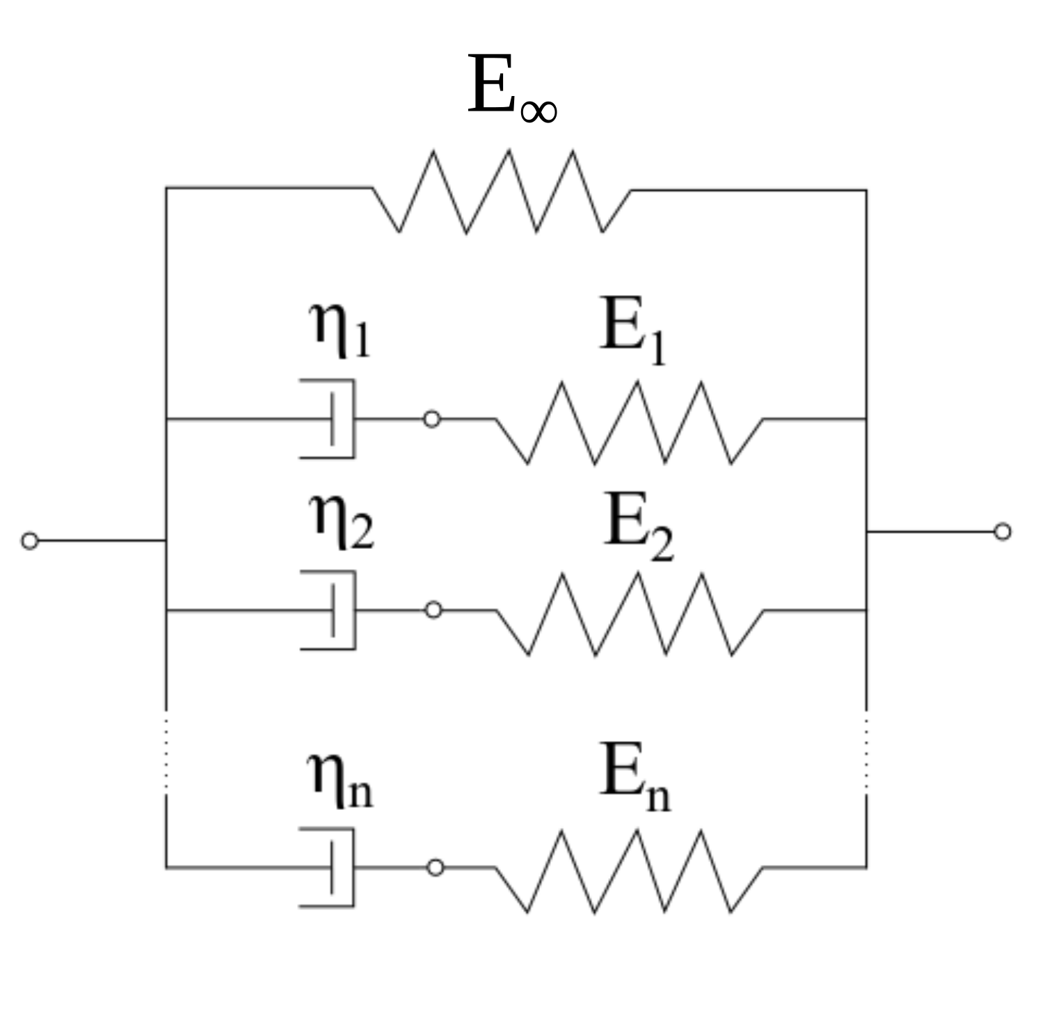
Fig. 19 Schematic representation of the Maxwell chain
A different visco-elastic rheological model available to users is the generalized Maxwell chain (see [dBvdB94] and Section 46.7.4 of [dia]). It consists of a series of sequential spring-dashpots (Maxwell elements) placed in parallel with one single spring (see Fig. 19). The relation between stresses and strain comes from
where \(E(t,\tau)\) is the time-dependent relaxation function, \(\tau\) is the loading age, and \(\mathbf{D}\) is the dimensionless matrix relating a 3D deformation state to a 1D relaxation function. The relaxation function is expanded in the exponential series
where the relaxation time of each Maxwell element is defined as \(\lambda_{\alpha}=\eta_{\alpha} / E_{\alpha}\) with \(\eta_{\alpha}\) being the viscosity of a dash-pot. Assuming a constant strain rate within each time step, the analytical integration of the right-hand side of Eq. 4 leads to the following form
with \(\sigma_{\alpha}(t)\) being the internal stress within each Maxwell element, defined as
The first term under the sum sign in above equation could be seen as the effective stiffness of a single Maxwell element multiplied by the matrix \(\mathbf{D}\) and the strain increment \(\Delta \varepsilon\):
Time increment \(Δt\) controls the rate dependency of the effective stiffness. By limit analysis, we find the limiting values of the effective stiffness which are equal to \(E_0\) for infinitely slow loading (\(Δt\) tending to infinity) and \(E_0+ΣE_α\) for infinitely fast (\(Δt\) tending to 0). At the end of each converged time step, the internal stress \(σ_α(t)\) is updated according to
The mandatory parameters for the material file are the following: rho
(density), nu (Poisson’s ratio), Plane_Stress (if set to zero plane
strain, otherwise plane stress), Einf (infinite time Young’s modulus),
Ev (Maxwell elements’ stiffness values stored in a vector), Eta
(dashpots’ viscosity values stored in a vector).
The Maxwell model is applied on the entire strain tensor and does not distinguish between its deviatoric and hydrostatic components. Note that the time step has to be specified for the model using current material both for static and dynamic simulations:
model.setTimeStep(time_step_value);
Plastic
Small-Deformation Plasticity
Keyword: plastic_linear_isotropic_hardening
Inherits from elastic
Material description with input file:
#input.dat

material plastic_linear_isotropic_hardening [
  name = material_name
  rho = 1000       # density (Real)
  E   = 2.1e9      # young's modulus (Real)
  nu = 0.4         # poisson's ratio (Real)
  h = 0.1          # Hardening modulus (Real)
  sigma_y = 1e6    # Yield stress (Real)
]
Energies:
potential: elastic part of the potential energyplastic: dissipated plastic energy (integrated over time)
The small-deformation plasticity is a simple plasticity material formulation which accounts for the additive decomposition of strain into elastic and plastic strain components. This formulation is applicable to infinitesimal deformation where the additive decomposition of the strain is a valid approximation. In this formulation, plastic strain is a shearing process where hydrostatic stress has no contribution to plasticity and consequently plasticity does not lead to volume change. Fig. 20 shows the linear strain hardening elasto-plastic behavior according to the additive decomposition of strain into the elastic and plastic parts in infinitesimal deformation as

Fig. 20 Stress-strain curve for the small-deformation plasticity with linear isotropic hardening.
In this class, the von Mises yield criterion is used. In the von Mises yield criterion, the yield is independent of the hydrostatic stress. Other yielding criteria such as Tresca and Gurson can be easily implemented in this class as well.
In the von Mises yield criterion, the hydrostatic stresses have no effect on the plasticity and consequently the yielding occurs when a critical elastic shear energy is achieved.
where \(\sigma_y\) is the yield strength of the material which can be function of plastic strain in case of hardening type of materials and \({\boldsymbol{\sigma}}^{{\mathrm{tr}}}\) is the deviatoric part of stress given by
After yielding \((f = 0)\), the normality hypothesis of plasticity determines the direction of plastic flow which is normal to the tangent to the yielding surface at the load point. Then, the tensorial form of the plastic constitutive equation using the von Mises yielding criterion (see equation 4.34) may be written as
In these expressions, the direction of the plastic strain increment (or equivalently, plastic strain rate) is given by \(\frac{{\boldsymbol{\sigma}}^{{\mathrm{tr}}}}{\sigma_{{\mathrm{eff}}}}\) while the magnitude is defined by the plastic multiplier \(\Delta p\). This can be obtained using the consistency condition which impose the requirement for the load point to remain on the yielding surface in the plastic regime.
Here, we summarize the implementation procedures for the small-deformation plasticity with linear isotropic hardening:
Compute the trial stress:
\[{\boldsymbol{\sigma}}^{{\mathrm{tr}}} = {\boldsymbol{\sigma}}_t + 2G\Delta \boldsymbol{\varepsilon} + \lambda \mathrm{tr}(\Delta \boldsymbol{\varepsilon})\boldsymbol{I}\]Check the Yielding criteria:
\[f = (\frac{3}{2} {\boldsymbol{\sigma}}^{{\mathrm{tr}}} : {\boldsymbol{\sigma}}^{{\mathrm{tr}}})^{1/2}-\sigma_y (\boldsymbol{\varepsilon}^p)\]Compute the Plastic multiplier:
\[\begin{split}\begin{aligned} d \Delta p &= \frac{\sigma^{tr}_{eff} - 3G \Delta P^{(k)}- \sigma_y^{(k)}}{3G + h}\\ \Delta p^{(k+1)} &= \Delta p^{(k)}+ d\Delta p\\ \sigma_y^{(k+1)} &= (\sigma_y)_t+ h\Delta p \end{aligned}\end{split}\]Compute the plastic strain increment:
\[\Delta {\boldsymbol{\varepsilon}}^p = \frac{3}{2} \Delta p \frac{{\boldsymbol{\sigma}}^{{\mathrm{tr}}}}{\sigma_{{\mathrm{eff}}}}\]Compute the stress increment:
\[{\Delta \boldsymbol{\sigma}} = 2G(\Delta \boldsymbol{\varepsilon}-\Delta \boldsymbol{\varepsilon}^p) + \lambda \mathrm{tr}(\Delta \boldsymbol{\varepsilon}-\Delta \boldsymbol{\varepsilon}^p)\boldsymbol{I}\]Update the variables:
\[\begin{split}\begin{aligned} {\boldsymbol{\varepsilon^p}} &= {\boldsymbol{\varepsilon}}^p_t+{\Delta {\boldsymbol{\varepsilon}}^p}\\ {\boldsymbol{\sigma}} &= {\boldsymbol{\sigma}}_t+{\Delta \boldsymbol{\sigma}} \end{aligned}\end{split}\]
We use an implicit integration technique called the radial return method to
obtain the plastic multiplier. This method has the advantage of being
unconditionally stable, however, the accuracy remains dependent on the step
size. The plastic parameters to indicate in the material file are:
\(\sigma_y\) (Yield stress) and h (Hardening modulus). In addition, the
elastic parameters need to be defined as previously mentioned: E (Young’s
modulus), nu (Poisson’s ratio).
Damage
In the simplified case of a linear elastic and brittle material, isotropic damage can be represented by a scalar variable \(d\), which varies from \(0\) to \(1\) for no damage to fully broken material respectively. The stress-strain relationship then becomes:
where \(\boldsymbol{\sigma}\),
\(\boldsymbol{\varepsilon}\) are the Cauchy stress and
strain tensors, and \(\boldsymbol{C}\) is the elastic
stiffness tensor. This formulation relies on the definition of an
evolution law for the damage variable. In Akantu, many possibilities
exist and they are listed below.
Marigo
Keyword: marigo
Inherits from elastic
Material description with input file:
#input.dat

material marigo [
  name = material_name
  rho = 1000           # density (Real)
  E   = 2.1e9          # young's modulus (Real)
  nu = 0.4             # poisson's ratio (Real)
  Plane_stress = false # Plane stress simplification (bool, only 2D problems)
  Yd = 0.1             # Hardening modulus (Random)
  Sd = 1.              # Damage energy (Real)
]
Energies:
dissipated: energy dissipated in damage
This damage evolution law is energy based as defined by Marigo [Mar81], [Lem96]. It is an isotropic damage law.
In this formulation, \(Y\) is the strain energy release rate, \(Y_d\) the rupture criterion and \(S\) the damage energy. The non-local version of this damage evolution law is constructed by averaging the energy \(Y\).
Mazars
Keyword: mazars
Inherits from elastic
Material description with input file:
#input.dat

material mazars [
   name = concrete
   rho = 3000        # density (Real)
   E   = 32e9        # young's modulus (Real)
   nu  = 0.2         # poisson's ratio (Real)
   K0  = 9.375e-5    # Damage threshold (Real)
   At  = 1.15        # Parameter damage traction 1 (Real)
   Bt  = 10000       # Parameter damage traction 2 (Real)
   Ac  = 0.8         # Parameter damage compression 1 (Real)
   Bc  = 1391.3      # Parameter damage compression 2 (Real)
   beta = 1.00       # Parameter for shear (Real)
]
Energies:
dissipated: energy dissipated in damage
This law introduced by Mazars [Maz84] is a behavioral model to represent damage evolution in concrete. This model does not rely on the computation of the tangent stiffness, the damage is directly evaluated from the strain.
The governing variable in this damage law is the equivalent strain \(\varepsilon_{{\mathrm{eq}}} = \sqrt{<\boldsymbol{\varepsilon}>_+:<\boldsymbol{\varepsilon}>_+}\), with \(<.>_+\) the positive part of the tensor. This part is defined in the principal coordinates (I, II, III) as \(\varepsilon_{{\mathrm{eq}}} = \sqrt{<\boldsymbol{\varepsilon_I}>_+^2 + <\boldsymbol{\varepsilon_{II}}>_+^2 + <\boldsymbol{\varepsilon_{III}}>_+^2}\). The damage is defined as:
With \(\kappa_0\) the damage threshold, \(A_t\) and \(B_t\) the damage parameter in traction, \(A_c\) and \(B_c\) the damage parameter in compression, \(\beta\) is the shear parameter. \(\alpha_t\) is the coupling parameter between traction and compression, the \(\varepsilon_i\) are the eigenstrain and the \(\varepsilon_{{\mathrm{nd}}\;i}\) are the eigenvalues of the strain if the material were undamaged.
The coefficients \(A\) and \(B\) are the post-peak asymptotic value and the decay shape parameters.
Non-Local Constitutive Laws
Continuum damage modeling of quasi-brittle materials undergo significant
softening after the onset of damage. This fast growth of damage causes a loss of
ellipticity of partial differential equations of equilibrium. Therefore, the
numerical simulation results won’t be objective anymore, because the dissipated
energy will depend on mesh size used in the simulation. One way to avoid this
effect is the use of non-local damage formulations. In this approach a local
quantity such as the strain is replaced by its non-local average, where the size
of the domain, over which the quantitiy is averaged, depends on the underlying
material microstructure. Akantu provides non-local versions of many
constitutive laws for damage. Examples are for instance the material
Mazars and the material
Marigo, that can be used in a non-local context. In
order to use the corresponding non-local formulation the user has to define the
non-local material he wishes to use in the text input file:
material constitutive_law_non_local [
    name = material_name
    rho = $value$
    ...
]
where constitutive_law_non_local is the name of the non-local constitutive law, e.g. marigo_non_local.
In addition to the material the non-local neighborhood, that should be used for the averaging process needs to be defined in the material file as well:
non_local neighborhood_name weight_function_type [
   radius = $value$
   ...
    weight_function weight_parameter [
      damage_limit = $value$
      ...
   ]
]
for the non-local averaging, e.g. base_wf, followed by the properties of the non-local neighborhood, such as the radius, and the weight function parameters. It is important to notice that the non-local neighborhood must have the same name as the material to which the neighborhood belongs!
The following two sections list the non-local constitutive laws and different type of weight functions available in Akantu.
subsection{Non-local constitutive laws}
Let us consider a body having a volume \(V\) and a boundary \(\Gamma\). The stress-strain relation for a non-local damage model can be described as follows:
with \(\vec{D}\) the elastic moduli tensor, \(\sigma\) the stress tensor, \(\epsilon\) the strain tensor and \(\bar{d}\) the non-local damage variable. Note that this stres-strain relationship is similar to the relationship defined in Damage model except \(\bar{d}\). The non-local damage model can be extended to the damage constitutive laws: Marigo and Mazars.
The non-local damage variable \(\bar{d}\) is defined as follows:
with \(W(\vec{x},\vec{y})\) the weight function which averages local damage variables to describe the non-local interactions. A list of available weight functions and its functionalities in akantu are explained in the next section.
Non-local weight functions
The available weight functions in Akantu are follows:
base_weight_function: This weight function averages local damage variables by using a bell-shape function on spatial dimensions.
damaged_weight_function: A linear-shape weight function is applied to average local damage variables. Its slope is determined by damage variables. For example, the damage variables for an element which is highly damaged are averaged over large spatial dimension (linear function including a small slope).
remove_damaged_weight_function: This weight function averages damage values by using a bell-shape function asbase_weight_function, but excludes elements which are fully damaged.
remove_damaged_with_damage_rate_weight_function: A bell-shape function is applied to average local damage variables for elements having small damage rates.
stress_based_weight_function: Non local integral takes stress states, and use the states to construct weight function: an ellipsoid shape. Detailed explanations of this weight function are given in Giry et al. [GD13].
Cohesive Constitutive laws
Linear Irreversible Law
Keyword: cohesive_linear
Material description with input file:
#input.dat

material cohesive_linear [
  name = cohesive
  sigma_c = 0.1                     # critical stress sigma_c  (default: 0)
  G_c = 1e-2                        # Mode I fracture energy
  beta = 0.                         # weighting parameter for sliding and normal opening (default: 0)
  penalty = 0.                      # stiffness in compression to prevent penetration (α in the text)
  kappa = 1.                        # ration between mode-I and mode-II fracture energy (Gc_II/Gc_I)
  contact_after_breaking = true     # Activation of contact when the elements are fully damaged
  max_quad_stress_insertion = false # Insertion of cohesive element when stress is high
                                    # enough just on one quadrature point
                                    # if false the average stress on facet's quadrature points is used
]

Fig. 21 Irreversible cohesive laws for explicit simulations.
Akantu includes the Snozzi-Molinari [SM13] linear irreversible cohesive law (see Fig. 21). It is an extension to the Camacho-Ortiz [CO96] cohesive law in order to make dissipated fracture energy path-dependent. The concept of free potential energy is dropped and a new independent parameter \(\kappa\) is introduced:
where \(G_\mathrm{c, I}\) and \(G_\mathrm{c, II}\) are the necessary works of separation per unit area to open completely a cohesive zone under mode I and mode II, respectively. Their model yields to the following equation for cohesive tractions \(\vec{T}\) in case of crack opening \({\delta}\):
where \(\sigma_\mathrm{c}\) is the material strength along the fracture, \(\delta_\mathrm{c}\) the critical effective displacement after which cohesive tractions are zero (complete decohesion), \(\Delta_\mathrm{t}\) and \(\Delta_\mathrm{n}\) are the tangential and normal components of the opening displacement vector \(\vec{\Delta}\), respectively. The parameter \(\beta\) is a weight that indicates how big the tangential opening contribution is. The effective opening displacement is:
In case of unloading or reloading \(\delta < \delta_\mathrm{max}\), tractions are calculated as:
so that they vary linearly between the origin and the maximum attained tractions. As shown in Fig. 21, in this law, the dissipated and reversible energies are:
Moreover, a damage parameter \(D\) can be defined as:
which varies from 0 (undamaged condition) and 1 (fully damaged condition). This variable can only increase because damage is an irreversible process. A simple penalty contact model has been incorporated in the cohesive law so that normal tractions can be returned in case of compression:
where \(\alpha\) is a stiffness parameter that defaults to zero. The relative contact energy is equivalent to reversible energy but in compression.
The material name of the linear decreasing cohesive law is
material_cohesive_linear and its parameters with their respective default
values are:
sigma_c = 0delta_c = 0beta = 0G_c = 0kappa = 1penalty = 0
where G_c corresponds to \(G_\mathrm{c, I}\). A random number
generator can be used to assign a random \(\sigma_\mathrm{c}\) to each
facet following a given distribution (see
Section Constitutive Laws). Only one parameter between delta_c
and G_c has to be specified. For random \(\sigma_\mathrm{c}\)
distributions, the chosen parameter of these two is kept fixed and the
other one is varied.
The bi-linear constitutive law works exactly the same way as the linear
one, except for the additional parameter delta_0 that by
default is zero. Two examples for the extrinsic and intrinsic cohesive
elements and also an example to assign different properties to
inter-granular and trans-granular cohesive elements can be found in
the folder examples/cohesive_element/.
Linear Cohesive Law with Friction
Keyword: cohesive_linear_friction
Material description with input file:
#input.dat


material cohesive_linear_friction [
  name = interface
  beta = 1                       # weighting parameter for sliding and normal opening (default: 0)
  G_c = 30e-3                    # Mode I fracture energy
  penalty = 1.0e6                # stiffness in compression to prevent penetration (α in the text)
  sigma_c = 2.0                  # critical stress sigma_c  (default: 0)
  contact_after_breaking = true  # Activation of contact when the elements are fully damaged
  mu = 0.5                       # Maximum value of the friction coefficient
  penalty_for_friction = 5.0e3   # Penalty parameter for the friction behavior
]
This law represents a variation of the linear irreversible cohesive of
the previous section, which adds friction. The friction behavior is
approximated with an elasto-plastic law, which relates the friction
force to the relative sliding between the two faces of the cohesive
element. The slope of the elastic branch is called
penalty_for_friction, and is defined by the user, together
with the friction coefficient, as a material property. The friction
contribution evolves with the damage of the cohesive law: it is null
when the damage is zero, and it becomes maximum when the damage is
equal to one. This is done by defining a current value of the
friction coefficient (mu) that increases linearly with the damage, up
to the value of the friction coefficient defined by the user. The
yielding plateau of the friction law is given by the product of the
current friction coefficient and the local compression stress acting
in the cohesive element. Such an approach is equivalent to a
node-to-node contact friction. Its accuracy is acceptable only for
small displacements.
The material name of the linear cohesive law with friction is
material_cohesive_linear_friction. Its additional parameters
with respect to those of the linear cohesive law without friction,
with the respective default values, are:
mu = 0penalty_for_friction = 0
Linear Cohesive Law with Fatigue
Keyword: cohesive_linear_fatigue
Material description with input file:
#input.dat

material cohesive_linear_fatigue [
      name = cohesive
      sigma_c = 1            # critical stress sigma_c  (default: 0)
      beta = 1               # weighting parameter for sliding and normal opening (default: 0)
      delta_c = 1            # Critical displacement
      delta_f = 1            # delta_f (normalization of opening rate to alter reloading stiffness after fatigue)
      count_switches = true  # Count the opening/closing switches per element
]
This law represents a variation of the linear irreversible cohesive law of the previous section, that removes the hypothesis of elastic unloading-reloading cycles. With this law, some energy is dissipated also during unloading and reloading with hysteresis. The implementation follows the work of [NROR01]. During the unloading-reloading cycle, the traction increment is computed as
where \(\dot{\delta}\) and \(\dot{T}\) are respectively the effective opening displacement and the cohesive traction increments with respect to time, while \(K^-\) and \(K^+\) are respectively the unloading and reloading incremental stiffness. The unloading path is linear and results in an unloading stiffness
where \(T_\mathrm{max}\) and \(\delta_\mathrm{max}\) are the maximum cohesive traction and the effective opening displacement reached during the precedent loading phase. The unloading stiffness remains constant during the unloading phase. On the other hand the reloading stiffness increment \(\dot{K}^+\) is calculated as
where \(\delta_\mathrm{f}\) is a material parameter (refer to [VRM15] for more details). During unloading the stiffness \(K^+\) tends to \(K^-\), while during reloading \(K^+\) gets decreased at every time step. If the cohesive traction during reloading exceeds the upper limit given by equation Eq. 5, it is recomputed following the behavior of the linear decreasing cohesive law for crack opening.
Exponential Cohesive Law
Keyword: cohesive_exponential
Material description with input file:
#input.dat

material cohesive_exponential [
  name = coh1
  sigma_c = 1.5e6             # critical stress sigma_c  (default: 0)
  beta = 1                    # weighting parameter for sliding and normal opening (default: 0)
  delta_c = 1e-4              # Critical displacement
  exponential_penalty = true  # Is contact penalty following the exponential law?
  contact_tangent = 1.0       # Ratio of contact tangent over the initial exponential tangent
]
Ortiz and Pandolfi proposed this cohesive law in 1999 [OP99b]. The traction-opening equation for this law is as follows:
This equation is plotted in Fig. 22. The term \(\partial{\vec{T}}/ \partial{\delta}\) after the necessary derivation can expressed as
where
As regards the behavior in compression, two options are available: a contact penalty approach with stiffness following the formulation of the exponential law and a contact penalty approach with constant stiffness. In the second case, the stiffness is defined as a function of the tangent of the exponential law at the origin.
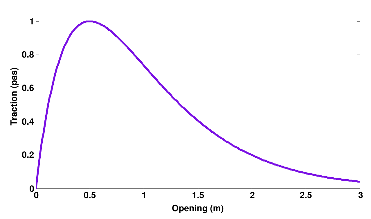
Fig. 22 Exponential cohesive law
Adding a New Constitutive Law
There are several constitutive laws in Akantu as described in the previous
Section Constitutive Laws. It is also possible to use a user-defined material
for the simulation. These materials are referred to as local materials since
they are local to the example of the user and not part of the Akantu
library. To define a new local material, two files (material_XXX.hh and
material_XXX.cc) have to be provided where XXX is the name of the new
material. The header file material_XXX.hh defines the interface of your
custom material. Its implementation is provided in the material_XXX.cc. The
new law must inherit from the Material class or
any other existing material class. It is therefore necessary to include the
interface of the parent material in the header file of your local material and
indicate the inheritance in the declaration of the class:
auto & solver = model.getNonLinearSolver();
solver.set("max_iterations", 1);
solver.set("threshold", 1e-4);
solver.set("convergence_type", SolveConvergenceCriteria::_residual);

model.solveStep();


/* ---------------------------------------------------------------------- */
#include "material.hh"
/* ---------------------------------------------------------------------- */

#ifndef AKANTU_MATERIAL_XXX_HH_
#define AKANTU_MATERIAL_XXX_HH_

namespace akantu {

class MaterialXXX : public Material {

/// declare here the interface of your material

};
In the header file the user also needs to declare all the members of the new material. These include the parameters that a read from the material input file, as well as any other material parameters that will be computed during the simulation and internal variables.
In the following the example of adding a new damage material will be
presented. In this case the parameters in the material will consist of the
Young’s modulus, the Poisson coefficient, the resistance to damage and the
damage threshold. The material will then from these values compute its Lamé
coefficients and its bulk modulus. Furthermore, the user has to add a new
internal variable damage in order to store the amount of damage at each
quadrature point in each step of the simulation. For this specific material the
member declaration inside the class will look as follows:
class LocalMaterialDamage : public Material {

/// declare constructors/destructors here

/// declare methods and accessors here

  /* -------------------------------------------------------------------- */
  /* Class Members                                                        */
  /* -------------------------------------------------------------------- */

  AKANTU_GET_MACRO_BY_ELEMENT_TYPE_CONST(Damage, damage, Real);
private:

  /// the young modulus
  Real E;

  /// Poisson coefficient
  Real nu;

  /// First Lame coefficient
  Real lambda;

  /// Second Lame coefficient (shear modulus)
  Real mu;

  /// resistance to damage
  Real Yd;

  /// damage threshold
  Real Sd;

  /// Bulk modulus
  Real kpa;

  /// damage internal variable
  InternalField<Real> damage;

};
In order to enable to print the material parameters at any point in the user’s example file using the standard output stream by typing:
for (Int m = 0; m  < model.getNbMaterials(); ++m)
  std::cout << model.getMaterial(m) << std::endl;
the standard output stream operator has to be redefined. This should be done at the end of the header file:
class LocalMaterialDamage : public Material {

  /// declare here the interace of your material

}:
/* ---------------------------------------------------------------------- */
/* inline functions                                                       */
/* ---------------------------------------------------------------------- */
/// standard output stream operator
inline std::ostream & operator <<(std::ostream & stream, const LocalMaterialDamage & _this)
{
  _this.printself(stream);
  return stream;
}
However, the user still needs to register the material parameters that
should be printed out. The registration is done during the call of the
constructor. Like all definitions the implementation of the
constructor has to be written in the material_XXX.cc
file. However, the declaration has to be provided in the
material_XXX.hh file:
class LocalMaterialDamage : public Material {
  /* -------------------------------------------------------------------- */
  /* Constructors/Destructors                                             */
  /* -------------------------------------------------------------------- */
public:

  LocalMaterialDamage(SolidMechanicsModel & model, const ID & id = "");
};
The user can now define the implementation of the constructor in the
material_XXX.cc file:
/* ---------------------------------------------------------------------- */
#include "local_material_damage.hh"
#include "solid_mechanics_model.hh"

namespace akantu {

/* ---------------------------------------------------------------------- */
LocalMaterialDamage::LocalMaterialDamage(SolidMechanicsModel & model,
           const ID & id)  :
  Material(model, id),
  damage("damage", *this) {
  AKANTU_DEBUG_IN();

  this->registerParam("E", E, 0., _pat_parsable, "Young's modulus");
  this->registerParam("nu", nu, 0.5, _pat_parsable, "Poisson's ratio");
  this->registerParam("lambda", lambda, _pat_readable, "First Lame coefficient");
  this->registerParam("mu", mu, _pat_readable, "Second Lame coefficient");
  this->registerParam("kapa", kpa, _pat_readable, "Bulk coefficient");
  this->registerParam("Yd", Yd,   50., _pat_parsmod);
  this->registerParam("Sd", Sd, 5000., _pat_parsmod);

  damage.initialize(1);

  AKANTU_DEBUG_OUT();
}
During the intializer list the reference to the model and the material id are
assigned and the constructor of the internal field is called. Inside the scope
of the constructor the internal values have to be initialized and the
parameters, that should be printed out, are registered with the function:
registerParam:
void registerParam(name of the parameter (key in the material file),
       member variable,
       default value (optional parameter),
       access permissions,
       description);
The available access permissions are as follows:
- _pat_internal: Parameter can only be output when the material is printed.
- _pat_writable: User can write into the parameter. The parameter is output when the material is printed.
- _pat_readable: User can read the parameter. The parameter is output when the material is printed.
- _pat_modifiable: Parameter is writable and readable.
- _pat_parsable: Parameter can be parsed, i.e. read from the input file.
- _pat_parsmod: Parameter is modifiable and parsable.
In order to implement the new constitutive law the user needs to specify how the additional material parameters, that are not defined in the input material file, should be calculated. Furthermore, it has to be defined how stresses and the stable time step should be computed for the new local material. In the case of implicit simulations, in addition, the computation of the tangent stiffness needs to be defined. Therefore, the user needs to redefine the following functions of the parent material:
void initMaterial();

// for explicit and implicit simulations void
computeStress(ElementType el_type, GhostType ghost_type = _not_ghost);

// for implicit simulations
void computeTangentStiffness(ElementType el_type,
           Array<Real> & tangent_matrix,
           GhostType ghost_type = _not_ghost);

// for explicit and implicit simulations
Real getStableTimeStep(Real h, const Element & element);
In the following a detailed description of these functions is provided:
initMaterial: This method is called after the material file is fully read and the elements corresponding to each material are assigned. Some of the frequently used constant parameters are calculated in this method. For example, the Lamé constants of elastic materials can be considered as such parameters.computeStress: In this method, the stresses are computed based on the constitutive law as a function of the strains of the quadrature points. For example, the stresses for the elastic material are calculated based on the following formula:\[\mat{\sigma } =\lambda\mathrm{tr}(\mat{\varepsilon})\mat{I}+2 \mu \mat{\varepsilon}\]Therefore, this method contains a loop on all quadrature points assigned to the material using the two macros:
MATERIAL_STRESS_QUADRATURE_POINT_LOOP_BEGINandMATERIAL_STRESS_QUADRATURE_POINT_LOOP_ENDMATERIAL_STRESS_QUADRATURE_POINT_LOOP_BEGIN(element_type); // sigma <- f(grad_u) MATERIAL_STRESS_QUADRATURE_POINT_LOOP_END;
The strain vector in Akantu contains the values of \(\nabla \vec{u}\), i.e. it is really the displacement gradient,
computeTangentStiffness: This method is called when the tangent to the stress-strain curve is desired (see Fig ref {fig:smm:AL:K}). For example, it is called in the implicit solver when the stiffness matrix for the regular elements is assembled based on the following formula:\[\label{eqn:smm:constitutive_elasc} \mat{K } =\int{\mat{B^T}\mat{D(\varepsilon)}\mat{B}}\]Therefore, in this method, the
tangentmatrix (mat{D}) is computed for a given strain.The
tangentmatrix is a \(4^{th}\) order tensor which is stored as a matrix in Voigt notation.
Fig. 23 Tangent to the stress-strain curve.
getCelerity: The stability criterion of the explicit integration scheme depend on the fastest wave celerity Explicit Time Integration. This celerity depend on the material, and therefore the value of this velocity should be defined in this method for each new material. By default, the fastest wave speed is the compressive wave whose celerity can be defined ingetPushWaveSpeed.
Once the declaration and implementation of the new material has been completed, this material can be used in the user’s example by including the header file:
#include "material_XXX.hh"
For existing materials, as mentioned in Constitutive Laws, by
default, the materials are initialized inside the method
initFull. If a local material should be used instead, the
initialization of the material has to be postponed until the local
material is registered in the model. Therefore, the model is
initialized with the boolean for skipping the material initialization
equal to true:
/// model initialization
model.initFull(_analysis_method = _explicit_lumped_mass);
Once the model has been initialized, the local material needs to be registered in the model:
model.registerNewCustomMaterials<XXX>("name_of_local_material");
Only at this point the material can be initialized:
model.initMaterials();
A full example for adding a new damage law can be found in
examples/new_material.
Adding a New Non-Local Constitutive Law
In order to add a new non-local material we first have to add the local
constitutive law in Akantu (see above). We can then add the non-local version
of the constitutive law by adding the two files (material_XXX_non_local.hh
and material_XXX_non_local.cc) where XXX is the name of the
corresponding local material. The new law must inherit from the two classes,
non-local parent class, such as the MaterialNonLocal class, and from the
local version of the constitutive law, i.e. MaterialXXX. It is therefore
necessary to include the interface of those classes in the header file of your
custom material and indicate the inheritance in the declaration of the class:
/* ---------------------------------------------------------------------- */
#include "material_non_local.hh" // the non-local parent
#include "material_XXX.hh"
/* ---------------------------------------------------------------------- */

#ifndef AKANTU_MATERIAL_XXX_HH_
#define AKANTU_MATERIAL_XXX_HH_

namespace akantu {

class MaterialXXXNonLocal : public MaterialXXX,
                            public MaterialNonLocal {

/// declare here the interface of your material

};
As members of the class we only need to add the internal fields to store the non-local quantities, which are obtained from the averaging process:
/* -------------------------------------------------------------------------- */
/* Class members                                                              */
/* -------------------------------------------------------------------------- */
protected:
  InternalField<Real> grad_u_nl;
The following four functions need to be implemented in the non-local material:
/// initialization of the material
void initMaterial();
/// loop over all element and invoke stress computation
virtual void computeNonLocalStresses(GhostType ghost_type);
/// compute stresses after local quantities have been averaged
virtual void computeNonLocalStress(ElementType el_type, GhostType ghost_type)
/// compute all local quantities
void computeStress(ElementType el_type, GhostType ghost_type);
In the intialization of the non-local material we need to register the local quantity for the averaging process. In our example the internal field grad_u_nl is the non-local counterpart of the gradient of the displacement field (grad_u_nl):
void MaterialXXXNonLocal::initMaterial() {
  MaterialXXX::initMaterial();
  MaterialNonLocal::initMaterial();
  /// register the non-local variable in the manager
  this->model->getNonLocalManager().registerNonLocalVariable(
    this->grad_u.getName(),
    this->grad_u_nl.getName(),
    spatial_dimension * spatial_dimension);
}
The function to register the non-local variable takes as parameters the name of the local internal field, the name of the non-local counterpart and the number of components of the field we want to average. In the computeStress we now need to compute all the quantities we want to average. We can then write a loop for the stress computation in the function computeNonLocalStresses and then provide the constitutive law on each integration point in the function computeNonLocalStress.
Contact Mechanics Model
The contact mechanics model is a specific implementation of
Model interface to handle contact between
bodies.
Theory
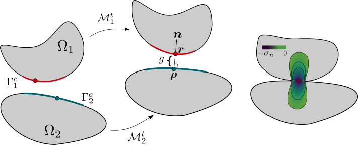
Fig. 24 Basic notation for the contact between two bodies.
Let us consider two deformable bodies, represented as \(\Omega_\alpha\), \(\alpha=1, 2\). The boundary \(\Gamma_\alpha\) of a body is divided into three non-intersecting regions : \(\Gamma^D_\alpha\) with prescribed displacements, \(\Gamma^N_\alpha\) with prescribed tractions and \(\Gamma^C_\alpha\) where the two bodies \(\Omega_1\) can potentially come into contact such that:
The motion of the two bodies is described in a fixed spatial frame defined by orthonormal basis \([\boldsymbol{e}_x, \boldsymbol{e}_y, \boldsymbol{e}_z]\) by mapping \(\mathcal{M}_\alpha^t\) in time interval \(t \in [0, T]\). In reference configuration \(i.e.~ t=0\), the position vector for an arbitrary point on body \(\Omega_\alpha\) is represented as \(\boldsymbol{X}_\alpha\) and in actual configuration the points are denoted by small letters for example \(\boldsymbol{x}\). Fig. 24 shows the motion of two bodies from the reference to actual configuration. During the motion, the bodies can potentially come in contact along \(\Gamma^C_\alpha\) as shown in Fig. 24, termed as potential contact zone. Upon contact, two physical conditions need to be satisfied \((i)\) the two surfaces \(\Gamma^C_\alpha\) cannot interpenetrate at any time during motion \((ii)\) forces must be exerted by bodies along the \(\Gamma^C_\alpha\) to resist the interpenetration as well as relative motion along the contacting surfaces. Of the two conditions, the non-penetration of bodies can be defined by a gap function \(g\) which represents the separation between the two bodies:
where \(\boldsymbol{r} \in \mathcal{M}[\Gamma^C_1]\) is the position of point \(\boldsymbol{X}_1\) at time \(t\) , \(\boldsymbol{\rho} \in \mathcal{M}[\Gamma^C_2]\) is the closest point projection of \(\boldsymbol{r}\) and \(\boldsymbol{n}\) is the outward normal at \(\boldsymbol{\rho}\) (see Fig. 24 b). To preclude the interpenetration, the gap function is constrained with \(g \geq 0\), as it is shown in Fig. 24 b. When the two bodies eventually come in contact, the gap vanishes \(i.e.~ g=0\) which leads to the development of tractions \(\boldsymbol{T}_\alpha\) along the contact interface. Thus, the boundary value problem can be formulated for the two bodies \(\Omega_\alpha\) with contact constraints as an extra boundary condition:
Solution spaces \(\mathcal{U}_\alpha\) and weighting spaces \(\mathcal{W}_\alpha\) are defined for each body:
The variational form for each body \(\alpha\) is given as
In equilibrium state, following Newton’s \(3^{rd}\) law, it can be stated the forces exerted by two bodies along \(\Gamma^C_\alpha\) are equal and opposite:
This allows to replace the two integrals over contact surfaces $Gamma^C_alpha$ with a single integral over any one of the surfaces:
The contact traction \(\boldsymbol{T}_1\) can be decomposed into its normal and tangential components as:
where \(\boldsymbol{T}^n\) is the component along the normal vector \(\boldsymbol{n}\) and \(\boldsymbol{T}^t\) is the component tangential to \(\boldsymbol{n}\) developed due to the friction along the surfaces. Upon contact , the normal pressure \(\sigma_n\) associated to \(\boldsymbol{T}^n\) must be compressive to preclude the interpenetration of bodies. In general, if a point is not in contact \(g > 0\), then \(\sigma_n=0\) and in contact \(\sigma_n < 0\). This leads to the non-penetration condition:
The above set of conditions care called Hertz-Signorini-Moreau or Karush-Kuhn-Tucker condition given as:
The tangential component of the contact traction is defined as :
where \(\boldsymbol{\sigma}\) is the Cauchy stress tensor and $boldsymbol{n}$ is the outward normal at \(\boldsymbol{\rho}\). The direction of tangential traction, \(\boldsymbol{s}\) is determined by the relative sliding velocity \(\boldsymbol{v}_t\) of the point \(\boldsymbol{r}\) and its projection point \(\boldsymbol{\rho}\) in contact and is given as:
According to the experimental observations of Amontons and [Cou21], in presence of friction, the interface develops a frictional strength which governs the sliding between them and thus constrains the tangential contact. In Akantu implementation, we restrict to the classical non-associated Coulomb’s friction law [Cou21] which is widely used in many physical and engineering applications. The Coulomb’s friction law, as a first-order approximation, states that the frictional strength is proportional to the normal pressure:
where \(\mu\) is coefficient of friction between interfaces. If the tangential traction \(||\boldsymbol{T}^t||\) developed is below the frictional strength, the relative tangential sliding is zero \(i.e.~\boldsymbol{v}_t = 0\) :
The above equation denotes a stick state. As soon as the tangential stress reaches the frictional strength, the two surfaces start slipping relative to each other \(i.e.~\boldsymbol{v}_t > 0\). The slipping of the surfaces ensures that the tangential stress does not exceeds the frictional strength, \(||\boldsymbol{\sigma}_t|| -\mu|\sigma_n| = 0\). This definition of slip state is defined as:
Similar to Karush-Kuhn-Tucker condition for normal contact, the above conditions formulate the necessary conditions for tangential contact:
The above contact and frictional constraints are unilateral in nature i.e. they do not behave symmetrically with respect to gap function, g. This renders the balance of work as a variational inequality:
which makes it a non-linear optimization problem. The strategy employed (optimization techniques) to find the solution of variational inequality depends on the choice of numerical framework employed to solve the B.V.P.
To solve the minimization problem, FEM introduces the concept of active set strategy to overcome the problem. In active set strategy, it is assumed that at current solution step, the part of potential contact zone \(\Gamma^C_1\) that are in contact are known, \(\Gamma^{C\star}_1 \subseteq \Gamma^C_1\). This is achieved by first allowing the two bodies to interpenetrate and finding the interpenetrated part of potential contact zone which will denote the active set. Knowing the active set, transforms the optimization problem to a variational equality where constraints are imposed along the active part of contacting interface:
Thus, the resolution of contact problem in FEM requires two steps: finding the active set along the contacting interface and then imposing the contact constraints along the active set only. In the following section, we describe how to employ the contact detection strategies implemented within Akantu in order to find the active set and to compute contact forces.
Using the Contact Mechanics Model
The ContactMechanicsModel
object solves the contact problem. An instance of
the class can be created like this:
ContactMechanicsModel contact(mesh, spatial_dimension);
while an existing mesh has been used (see sect-common-mesh). To intialize the model object:
contact.initFull(_analysis_method = _explicit_lumped_mass);
The contact mechanics model contains Arrays:
gapscontains the nodal interpenetrating value \(g\) (positive for interpenetration, zero by default after initialization)
normalscontains the normal vector at the slave nodes (zero by default after initialization).
In Akantu, the possible contact between surfaces is divided into 3 categories.
Physical Surfaces - The contact occurs between two pyhsically defined boundaries/surfaces of a body.
Cohesive Surfaces - The contact occurs between fracturing surfaces created using
SolidMechanicsModelCohesive.All Surfaces - The contact can occur between physical as well as cohesive surfaces.
To select the contacting surfaces, one must define a
SurfaceSelector of one of the
above defined types.
To define contact between Physical surfaces, an instance of
PhysicalSurfaceSelector
is created where the mesh object (see sect-common-mesh) is
passed as an argument:
auto && surface_selector = std::make_shared<PhysicalSurface>(mesh);
To define contact between cohesive surfaces, an instance of
CohesiveSurfaceSelector
must be created. As the contact occurs between the cohesive facets,
therefore the mesh facet object is passed as an argument:
auto && surface_selector = std::make_shared<CohesiveSurface>(mesh.getMeshFacets());
To defind contact between physical and cohesive surfaces, an instance of
AllSurfaceSelector
must be created. As the contact occurs between the cohesive facets,
therefore the mesh facet object is passed as an argument:
auto && surface_selector = std::make_shared<AllSurface>(mesh.getMeshFacets());
Once a surface selector is created it must be assigned to the
ContactDetector class:
contact.getContactDetector().setSurfaceSelector(surface_selector);
Contact detection
The contact detection algorithm can receive a few parameters. It is possible to specify the master/slave surfaces with their string identifier. The geometrical projections are performed with iterations which can be controlled as a classical optimization problem. A typical detection configuration is given below:
contact_detector [
  type = explicit
  master = contact_bottom
  slave = contact_top
  projection_tolerance = 1e-10
  max_iterations = 100
  extension_tolerance = 1e-5
]
Contact resolution
The contact resolution defines the surface tractions due to contact both for normal and tangential contact. A typical configuration for a penalization formulation is as follows:
contact_resolution penalty_linear [
  name = contact_top
  mu = 0.0                      # friction coefficient
  epsilon_n = 4e5               # normal penalization
  epsilon_t = 1e5               # friction penalization
  is_master_deformable = false  # when master is rigid => computational savings
]
Coupling with SolidMechanicsModel
To couple the
ContactMechancisModel
contact mechanics model with
SolidMechanicsModel a
dedicated coupler class CouplerSolidContact is provided.
When an instance of a coupler class is created, it automatically creates the instances of solid mechanics model and contact mechanics model. The two objects can be retrived from the coupler class.
CouplerSolidContact coupler(mesh);
auto & solid = coupler.getSolidMechanicsModel();
auto & contact = coupler.getContactMechanicsModel();
Simply initializing the coupler initializes the two models.
coupler.initFull( _analysis_method = _explicit_lumped_mass);
However to set the material selector and the contact detector for the two models, one must set them using directly the instance of the two model classes.
auto && selector = std::make_shared<MeshDataMaterialSelector<std::string>>(
                  "physical_names",solid);
solid.setMaterialSelector(selector);
auto && surface_selector = std::make_shared<PhysicalSurfaceSelector>(mesh);
contact.getContactDetector().setSurfaceSelector(surface_selector);
The dumping fields/vectors belonging to the solid mechanics model and contact mechanics model can directly be set through the coupler class.
coupler.setBaseName("contact-explicit-dynamic");
coupler.addDumpFieldVector("displacement");
coupler.addDumpFieldVector("normal_force");
coupler.addDumpFieldVector("external_force");
coupler.addDumpFieldVector("internal_force");
coupler.addDumpField("gaps");
coupler.addDumpField("areas");
coupler.addDumpField("stress");
Finally to solve the two models solveStep function of coupler class must be
invoked.
coupler.solveStep();
Coupling with SolidMechanicsModelCohesive
To use the contact mechanics model with cohesive elements, one must use the
CouplerSolidCohesiveContact to
coupler the ContactMechancisModel
with
SolidMechanicsModelCohesive.
The initialization and invocation of the functions are similar to
CouplerSolidContact except a few
changes.
solid = coupler.getSolidMechanicsModelCohesive();
While initializing the coupler, the nature of cohesive elements (extrinsic/intrinsic) should need to be passed.
coupler.initFull( _analysis_method = _explicit_lumped_mass, _is_extrinsic=true);
To ensure that cohesive elements break during an explicit insertion, one must
call the function checkCohesiveStress() after
solveStep().
coupler.solveStep();
solid.checkCohesiveStress();
Models [Unstable]
This models are implemented for some research purposes but might not have the same level of stability or tests than the models that are not marked unstable.
Diffusion Model
The heat transfer model is a specific implementation of the Model interface dedicated to handle the dynamic heat equation.
Theory
The strong form of the dynamic heat equation can be expressed as:
with \(T\) the scalar temperature field, \(c_v\) the specific heat capacity, \(\rho\) the mass density, \(\mat{\kappa}\) the conductivity tensor, and \(b\) the heat generation per unit of volume. The discretized weak form with a finite number of elements is
with \(i\) and \(j\) the node indices, \(\vec{n}\) the normal field to the surface \(\Gamma = \partial \Omega\). To simplify, we can define the capacity and the conductivity matrices as
and the system to solve can be written:
with \(\vec{Q}^{\text{ext}}\) the consistent heat generated.
The diffusion model is meant as a base to implement different diffusive processes, heat diffusion, chemical diffusion, simple flow problems, etc. Currently only one of this physics is implemented, the heat diffusion, in a model named HeatTransferModel
Using the Heat Transfer Model
A material file name has to be provided during initialization.
Currently, the HeatTransferModel object uses dynamic analysis
with an explicit time integration scheme. It can simply be created
like this
HeatTransferModel model(mesh, spatial_dimension);
while an existing mesh has been used (see sect-common-mesh). Then the model object can be initialized with:
model.initFull()
This function will load the material properties, and allocate / initialize the
nodes and element Arrays. The solver type and its
parameters can also be configured directly in the input file — see
Model solver configuration.
More precisely, the heat transfer model contains 4 Arrays:
temperature contains the nodal temperature \(T\) (zero by default after the initialization).
temperature_rate contains the variations of temperature \(\dot{T}\) (zero by default after the initialization).
blocked_dofs contains a Boolean value for each degree of freedom specifying whether the degree is blocked or not. A Dirichlet boundary condition (\(T_d\)) can be prescribed by setting the blocked_dofs value of a degree of freedom to
true. The temperature and the temperature_rate are computed for all degrees of freedom where the blocked_dofs value is set tofalse. For the remaining degrees of freedom, the imposed values (zero by default after initialization) are kept.external_heat_rate contains the external heat generations. \(\vec{Q^{ext}}\) on the nodes.
internal_heat_rate contains the internal heat generations. \(\vec{Q^{int}} = -\mat{K} \cdot \vec{T}\) on the nodes.
Only a single material can be specified on the domain. A material text file (e.g. material.dat) provides the material properties as follows:
model heat_transfer_model [
  constitutive_law heat_diffusion [
    name = %\emph{XXX}%
    capacity = %\emph{XXX}%
    density = %\emph{XXX}%
    conductivity = [%\emph{XXX}% ... %\emph{XXX}%]
  ]
]
where the capacity and density are scalars, and the conductivity is
specified as a \(3\times 3\) tensor.
Explicit Dynamic
The explicit time integration scheme in Akantu uses a lumped capacity matrix
\(\mat{C}\) (reducing the computational cost, see Chapter Solid Mechanics Model / Solid Mechanics Model Cohesive).
This matrix is assembled by distributing the capacity of each element onto its
nodes. Therefore, the resulting \(\mat{C}\) is a diagonal matrix stored in
the capacity Array of the model.
model.assembleCapacityLumped();
Note
Currently, only the explicit time integration with lumped capacity
matrix is implemented within Akantu.
The explicit integration scheme is Forward Euler [Cur92].
Predictor: \(\vec{T}_{n+1} = \vec{T}_{n} + \Delta t \dot{\vec{T}}_{n}\)
Update residual: \(\vec{R}_{n+1} = \left( \vec{Q^{ext}_{n+1}} - \vec{K}\vec{T}_{n+1} \right)\)
Corrector : \(\dot{\vec{T}}_{n+1} = \mat{C}^{-1} \vec{R}_{n+1}\)
The explicit integration scheme is conditionally stable. The time step has to be
smaller than the stable time step, and it can be obtained in Akantu as
follows:
time_step = model.getStableTimeStep();
The stable time step is defined as:
where \(\Delta x\) is the characteristic length (e.g the in-radius in the case of linear triangle element), \(\rho\) is the density, \(\mat{\kappa}\) is the conductivity tensor, and \(c_v\) is the specific heat capacity. It is necessary to impose a time step which is smaller than the stable time step, for instance, by multiplying the stable time step by a safety factor smaller than one.
const Real safety_time_factor = 0.1;
Real applied_time_step = time_step * safety_time_factor;
model.setTimeStep(applied_time_step);
The following loop allows, for each time step, to update the temperature,
residual and temperature_rate fields following the previously described
integration scheme.
for (Int s = 1; (s-1)*applied_time_step < total_time; ++s) {
  model.solveStep();
}
An example of explicit dynamic heat propagation is presented in
examples/heat_transfer/explicit_heat_transfer.cc. This example consists
of a square 2D plate of \(1 \text{m}^2\) having an initial temperature of
\(100 \text{K}\) everywhere but a none centered hot point maintained at
\(300 \text{K}\). Fig. 25 presents the geometry
of this case. The material used is a linear fictitious elastic material with a
density of \(8940 \text{kg}/\text{m}^3\), a conductivity of
\(401 \text{W}/\text{m}/\text{K}\) and a specific heat capacity of
\(385 \text{J}/\text{K}/\text{kg}\). The time step used is
\(0.12 \text{s}\).

Fig. 25 Initial temperature field

Fig. 26 Temperature field after 15000 time steps = 30 minutes. The lines represent iso-surfaces.
PhaseField Model
The phasefield model is a specific implementation of
Model interface to handle brittle fracture
for infinitesimal strains.
Theory
The variational formulation of brittle fracture was first proposed by Francfort and Marigo [FM98] so as to overcome the shortcomings of Griffith’s criteria. The approach used by Francfort and Margio for variational formulation is based on the principle of global minimality of total energy. Similar to Griffith’s work, they define a surface energy corresponding to the discontinuity \(\Gamma\) as
where \(\mathcal{H}^{d-1}\) is d-1 dimensional Hausdroff measure which is surface measure for smooth hypersurfaces. the material behavior is considered to be linearly elastic with small strains throughout the body. Based on these assumptions the elastic energy of the body is defined as
where \(\psi\) is elastic energy density and it is given as a function of strain as
Exponential phasefield law
Bourdin et. al. [BFM00] in their work proposed a regularized version of variational formulation where a scalar field variable \(d(\vec{x},t)\) is used to represent crack. This scalar field variable approximates the sharp crack topology by taking value 1 at crack location and smoothly diffusing into value 0 away from the crack. figref{fig:diffusive_topology} shows both sharp crack topology and an approximated regularized crack topology for one-dimensional case.
The strong form of the phasefield can be expressed as
Using the PhaseField Model
The PhaseFieldModel object
solves the strong form using an inplicit solver. An instance of the
class can be created like this:
PhaseFieldModel phase(mesh, spatial_dimension);
while ans existing mesh has been used (see sect-common-mesh). To intialize the model object:
phase.initFull();
Currently, only an implicit solver is defined for the phasefield model. By default it is of linear type; it can be changed to a non-linear solver by initiating a new solver type. The solver type and its parameters can also be configured directly in the input file — see Model solver configuration.
The phasefield model contains Arrays:
damage:contains the nodal damage \(d\) (zero by default after the initialization)
blocked_dofscontains a Boolean value specifying whether the damage at a node is to be blocked or not. A Dirichlet boundary condition can be prescribed by setting the blocked_dofs value of damage to
true. The damage ais computed for all nodes where the blocked_dofs value is set tofalse. For the remaining nodes, the imposed values (zero by default after initialization) are kept.internal_forcecontains the driving force responsible for the crack to nucelate or propagate.
Currently, the phasefield model uses a exponential shaped scalar field variable \(d(\vec{x}, t)\) to approximate the sharp crack topology. A Phasefield variable thus requires a length scale parameter \(l_0\) to control the width of the diffusive crack topology along with the material parameters such as elastic modulus, poisson’s ratio, critical energy release rate.
The data input file provides the parameters for the exponential phasefield law as follows:
phasefield exponential [
           name = plate
           E = 210.0
           nu =  0.3
           gc = 5e-3
           l0 = 0.1
]
PhaseFieldModelcan handlephasefield laws for multiple materials. To define so:
phasefield exponential [
           name = hard
           E = 210.0
           nu =  0.3
           gc = 5e-3
           l0 = 0.1
]

phasefield exponential [
           name = soft
           E = 21.0
           nu =  0.3
           gc = 5e-5
           l0 = 0.1
]
In order to assign correct phasefield variable properties based on the
names of region as defined in mesh file,
MeshDataPhaseFieldSelector must be set as phasefield
selector:
auto && selector = std::make_shared<MeshDataPhaseFieldSelector<std::string>>(
        "physical_names", phase);
phase.setPhaseFieldSelector(selector);
For the crack to nucleate or propagate, phasefield model requires
strain measure at each quadrature point. The strain measure computed
from solid mechanics model is provided to the phasefield
model. Similarly, damage value computed at each quadrature point by
the phasefield model is provided to the solid mechanics model. This
damage is thus used to degrade the the elastic strain energy. To do
so, a new material which is a specific implementation of
MaterialDamage is defined for
solid mechanics model. The governing equation is given as
where \(\psi\) is the elastic energy and \(\eta\) is a numerical parmaeter avoid numerical difficulties due to full degradation of elastic energy for fully broken state. The material properties are thus provided in the input data filled as:
material phasefield [
      name = hard
      rho = 1.
      E = 210.0
      nu = 0.3
      eta = 0.0
      Plane_Stress = false
]

material phasefield [
      name = soft
      rho = 1.
      E = 21.0
      nu = 0.3
      eta = 0.0
      Plane_Stress = false
]
To simplify the execution of phasefield model coupled with
solidmechanis model, a special class
CouplerSolidPhaseField is
provided.
Coupling Phase Field Model and Solid Mechanics Model
A dedicated coupler class CouplerSolidPhaseField is defined in Akantu to ease the
coupling of the two models.
When an instance of a Coupler class is created, it automatically creates the instances of solid mechanics model and phasefield model. The two objects can be retrived from the coupler class.
CouplerSolidPhaseField coupler(mesh);
auto & phase = coupler.getPhaseFieldModel();
auto & solid = coupler.getSolidMechanicsModel();
The two objects must be used to define the solver type and apply boundary conditions.
solid.initFull(_analysis_method = _explicit_lumped_mass);
phase.initFull(_analysis_method = _static);
The whole process of coupling the two models at a given time step is
made easy by the solve
function of coupler class.
coupler.solve(<solver_id_for_solid_model>, <solver_id_for_phasefield_model>);
Staggered scheme
To solve the solid mechanics model and phasefield model, staggered scheme is implemented. In staggered scheme, at current time step first solid mechanics model is solved assuming the damage values from the previous time step. The strain thus computed are passed to the phasefield model and now, phasefield model is solved for the damage variable. At each iteration step, convergence in displacement and damage is checked for. If convergence is not reached, the combined newton-raphson iteration continues.
To illustrate the staggered scheme solution of phasefield model, one can refere to the examples provided for the phasefield model. Two examples provided are for static phasefield-static.py and dynamic crack propgation phasefield-dynamic.py.
For the static problem, both the solid mechanics model and the phsefield model are solved using alinear implicit solver. Convergence in value of both displacement as well as damage is checked at each loading step.
In case of the dynamic problem, solid mechanics model is solved dynamically using an explicit solver and the phasefield model is solved using a linear implcit solver. In this sceanrio, the staggered scheme doesnot check for any convergence. Below is the crack propagation observed for the dyanmic problem.
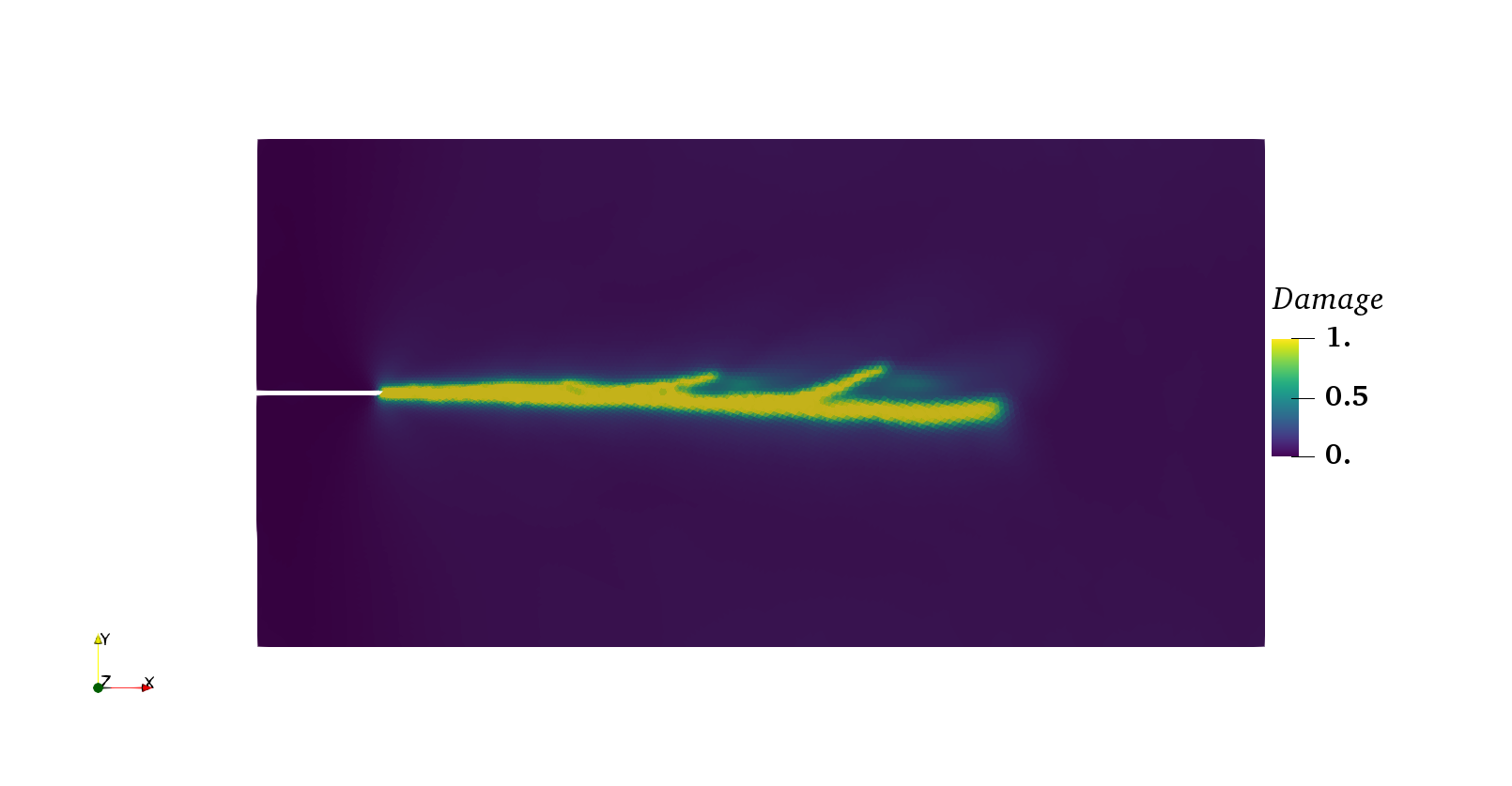
Fig. 27 Dynamic crack propagation using phasefield model
Structural Mechanics Model
Static structural mechanics problems can be handled using the class
StructuralMechanicsModel. So
far, Akantu provides 2D and 3D Bernoulli beam elements [FJ09].
This model is instantiated for a given Mesh, as for
the SolidMechanicsModel. The model
will create its own FEEngine object to compute
the interpolation, gradient, integration and assembly operations. The
StructuralMechanicsModel
constructor is called in the following way:
StructuralMechanicsModel model(mesh, spatial_dimension);
where mesh is a Mesh object defining the structure for
which the equations of statics are to be solved, and
spatial_dimension is the dimensionality of the problem. If
spatial_dimension is omitted, the problem is assumed to have
the same dimensionality as the one specified by the mesh.
Warning
Dynamic computations are not supported to date.
Note
Structural meshes are created and loaded
with _miot_gmsh_struct instead of _miot_gmsh (cf. Creating and Loading a Mesh)
Mesh mesh;
mesh.read("structural_mesh.msh", _miot_gmsh_struct);
This model contains at least the following Arrays:
blocked_dofs contains a Boolean value for each degree of freedom specifying whether that degree is blocked or not. A Dirichlet boundary condition can be prescribed by setting the blocked_dofs value of a degree of freedom to
true. The displacement is computed for all degrees of freedom for which the blocked_dofs value is set tofalse. For the remaining degrees of freedom, the imposed values (zero by default after initialization) are kept.displacement_rotation contains the generalized displacements (i.e. displacements and rotations) of all degrees of freedom. It can be either a computed displacement for free degrees of freedom or an imposed displacement in case of blocked ones (\(\vec{u}\) in the following).
external_force contains the generalized external forces (forces and moments) applied to the nodes (\(\vec{f_{\st{ext}}}\) in the following).
internal_force contains the generalized internal forces (forces and moments) applied to the nodes (\(\vec{f_{\st{int}}}\) in the following).
An example to help understand how to use this model will be presented in the next section.
Model Setup
Initialization
The easiest way to initialize the structural mechanics model is:
model.initFull();
The method initFull computes the shape
functions, initializes the internal vectors mentioned above and allocates the
memory for the stiffness matrix, unlike the solid mechanics model, its default
argument is _static.
Material properties are defined using the StructuralMaterial structure described in
Table 6. Such a definition could, for
instance, look like
StructuralMaterial mat1;
mat.E=3e10;
mat.I=0.0025;
mat.A=0.01;
Field |
Description |
|---|---|
|
Young’s modulus |
|
Cross section area |
|
Second cross sectional moment of inertia (for 2D elements) |
|
|
|
|
|
Polar moment of inertia of beam cross section (for 3D elements) |
Materials can be added to the model’s element_material vector using
model.addMaterial(mat1);
They are successively numbered and then assigned to specific elements.
for (Int i = 0; i < nb_element_mat_1; ++i) {
  model.getElementMaterial(_bernoulli_beam_2)(i,0) = 1;
}
Setting Boundary Conditions
As explained before, the Dirichlet boundary conditions are applied through the
array blocked_dofs. Two options exist to define Neumann conditions.
If a nodal force is applied, it has to be directly set in the array
force_momentum. For loads distributed along the beam length, the
method computeForcesFromFunction integrates them into nodal forces. The
method takes as input a function describing the distribution of loads along the
beam and a functor BoundaryFunctionType specifing if the function is expressed in the local coordinates (_bft_traction_local) or in the
global system of coordinates (_bft_traction).
static void lin_load(double * position, double * load,
                     Real * normal, UInt surface_id){
  memset(load,0,sizeof(Real)*3);
  load[1] = position[0]*position[0]-250;
}
int main(){
  ...
  model.computeForcesFromFunction<_bernoulli_beam_2>(lin_load,
                                                     _bft_traction_local);
  ...
}
Static Analysis
The StructuralMechanicsModel class can perform static analyses of structures. In this case, the equation to solve is the same as for the SolidMechanicsModel used for static analyses
where \(\mat{K}\) is the global stiffness matrix, \(\vec{u}\) the generalized displacement vector and \(\vec{f_{\st{ext}}}\) the vector of generalized external forces applied to the system.
To solve such a problem, the static solver of the
StructuralMechanicsModel object
is used. First a model has to be created and initialized.
StructuralMechanicsModel model(mesh);
model.initFull();
model.initFullinitializes all internal vectors to zero.
Note
The solver type and its parameters can also be configured directly in the input file. See Model solver configuration for the full syntax.
Once the model is created and initialized, the boundary conditions can be set as explained in Section Setting Boundary Conditions. Boundary conditions will prescribe the external forces or moments for the free degrees of freedom \(\vec{f_{\st{ext}}}\) and displacements or rotations for the others. To completely define the system represented by equation (Eq. 9), the global stiffness matrix \(\mat{K}\) must be assembled.
model.assembleStiffnessMatrix();
The computation of the static equilibrium is performed using the same Newton-Raphson algorithm as described in Static Analysis.
note{To date, StructuralMechanicsModel handles only constitutively and
geometrically linear problems, the algorithm is therefore guaranteed to converge
in two iterations.}
model.solveStep();
model.solveStepsolves the Eq. 9. The increment vector of the model will contain the new increment of displacements, and the displacement_rotation vector is also updated to the new displacements.
At the end of the analysis, the final solution is stored in the
displacement_rotation vector. A full example of how to solve a structural
mechanics problem is presented in the code
example/structural_mechanics/bernoulli_beam_2_example.cc. This example is
composed of a 2D beam, clamped at the left end and supported by two rollers as
shown in Fig. 28. The problem is defined by the
applied load \(q=6 \text{kN/m}\), moment \(\bar{M} = 3.6 \text{kN m}\),
moments of inertia \(I_1 = 250\,000 \text{cm}^4\) and \(I_2 = 128\,000
\text{cm}^4\) and lengths \(L_1 = 10\text{m}\) and \(L_2 = 8\text{m}\).
The resulting rotations at node two and three are \(\varphi_2 = 0.001\,167\)
and \(\varphi_3 = -0.000\,771\).

Fig. 28 2D beam example
Node To Node Contact
The node to node (NTN) contact model handles the interaction between two contacting surfaces, the bodies in contact being described by a SolidMechanicsModel.
Using the Node To Node Contact Model
To use the node to node contact, a dedicated coupler class NTNContactSolverCallback is provided.
To instantiate a coupler object, one needs to pass a solid mechanics model object SolidMechanicsModel, the ID of the geometrical boundaries constituting the two sides of the interface, the orientation of the normal surface and the time step factor to be used in the dynamic computation. A schematic showing the interfaces between two meshes (bottom one in black, top one in brown) is shown in Fig. 29. The coupler applies opposite forces on the matching nodes and couple the two surfaces together. The interfacial forces are limited by the chosen constitutive behavior (see Interfacial constitutive behavior) such that displacement discontinuities can develop between the two surfaces.
NTNContactSolverCallback coupler(solid,slave,master,surface_nor_dir,time_step)
Fig. 29 Contact interface between two bodies. The bottom (black, -) and top (brown, +) have matching nodes on the contacting surfaces of normal \(\vec{n}_{\pm}\). Normal \(\vec{f}_{\mathrm N,\pm}\) and frictional forces \(\vec{f}_{\mathrm T,\pm}\) are applied on the matching nodes, whose area of influence is indicated by \(A\).
Implementation
The residual on nodes part of the contact interface can be written as :
with \(\vec{f}_{\mathrm{N}}\) and \(\vec{f}_{\mathrm{T}}\) respectively the contact and the frictional forces at the contact interface. Note that they are zero for any nodes that are not on the interface.
Contact forces
The contact forces are computed based on a non overlapping condition in the normal direction:
where \([\![\vec{x}]\!]\) indicates the difference between the jump in fields between the nodal position \(x\) of the node in the top body and its matching node in the bottom body, and the subscript \(\rm N\) the normal direction. The non overlapping condition can be expressed as:
The gap in displacement \([\![\vec{u}]\!]_{\rm N}^{\rm i+2}\) can be expressed as the gap in the fields at the previous time step:
Replacing the velocity by its expression based on the predicted velocity and the acceleration increment, one gets
Replacing \([\![\ddot{\vec{\delta u}}]\!]_{\rm N}^{i}\) by \([\![\ddot{\vec{u}}]\!]_{\rm N}^{i} - [\![\ddot{\vec{u}}]\!]_{\rm N}^{i-1}\), and using Eq. 10 results in:
Let us define \([\![\ddot{\vec{u}}^{free}]\!]_{\rm N}^{i} = \mat{M}^{-1} \left([\![\vec{f}_{\mathrm{ext}}]\!]^{i} - [\![\vec{f}_{\mathrm{int}}]\!]^{i} \right)\) the acceleration related to the residual of the bodies that are not related by the node to node algorithm. The contact forces can be written as \([\![\vec{f}]\!]_{\rm N}^{i} = \vec{A} [\![\vec{T}]\!]_{\rm N}^{i}\) with \(\vec{A}\) the area associated to the contact nodes, and \(\vec{T}_{\rm N}^{\rm i}\) the contact stress. As the stress on the top and bottom matching nodes are equal and opposites, one can replace \([\![\vec{T}]\!]_{\rm N}^{i}\) by \(-2\vec{T}_{\rm N}^{i}\). Let us introduce the variable \(\vec{Z}\) :
We can then simplify Eq. 12 as:
In Eq. 13 all the terms except one are independent of the node to node algorithm. Let us introduce a last variable \(I^{free}\), that we call here the interpenetration of the free bodies:
Then, if \({\vec{I}^{free}}^{i} \geq 0\), it means that there is no need for corrective contact stress to forbid interpenetration, and thus \(\vec{T}_{\rm N}^{i}=0\). However, if \({\vec{I}^{free}}^{i} \leq 0\), then the contact stresses need to be computed as:
and the forces are then applied on the nodes as:
Friction forces
For the tangential (friction) forces, a similar derivation is done, but this time starting with a condition on the relative velocity in the tangential direction of the matching nodes at the mid-time step. This first condition assumes that the friction forces are sufficient to hold the body together and thus there is no gap in velocity:
The velocity at the mid-time step is given by \(\dot{\vec{u}}_{\rm T}^{i+1/2} = \dot{\vec{u}}_{\rm T}^{i} + \ddot{\vec{u}}_{\rm T}^{i} \Delta t /2\). Thus, we can write:
Defining \([\![\vec{f}]\!]_{\rm T}^{i} = \vec{A} [\![\vec{T}]\!]_{\rm T}^{i}\) and using the argument that the frictional stresses are equal and opposite \([\![\vec{T}]\!]_{\rm T}^{i}\) by \(-2\vec{T}_{\rm T}^{i}\), we can write:
Similarly to the case of contact forces, let us introduce \(\vec{R}^{free}\) as:
The tangential stress required to forbid any relative movement between two matching nodes is then given by:
and the corresponding force applied on the nodes:
The constitutive behavior of the frictional interfaces determines if these forces are applied in full or not, depending on the frictional strength of the interface \(\vec{S}_{\rm T}^{i}\), the forces added to the residual being given by \(\vec{A} min(\vec{T}_{\rm T},\vec{S}_{\rm T})\). The constitutive behavior currently implemented in akantu are described in the next section.
Interfacial constitutive behavior
Friction laws
Rate and state
in which \(\mu(v,\phi)\) is the friction coefficient given by a rate and state friction formulation and \(\phi\) is the state variable representing the age of contact. The velocity used to evaluate \(\mu\) is the relative velocity between the two surfaces, \(v = [\![\dot{\vec{u}}]\!]_{\rm T}\).
For rate and state friction, the time step have to be significantly reduced compared to regular bulk finite element simulations, see [RBBM20]. For the typical simulations with node to node contact described by rate and state friction laws, the safety factor for the time step should be around \(\alpha_{\rm F} = \mathcal{O}(0.01)\).
The updated explicit scheme relies on adding both the contact and the frictional forces \(\vec{f}_{\rm N}^{i}\) and \(\vec{f}_{\rm T}^{i}\) when the residual is evaluated, by using Eq. 10 to compute the acceleration increment.
Rate evolution laws
Dieterich law
The classical law proposed by Dietriech and Ruina.
Revised Dieterich law
A “+1” term is added inside the log of velocity to avoid NaN values when the velocity tends toward 0. Note the \(b \mu_0\) to have a coherent shape with the N-shaped law.
Regularised Dieterich law
A “+1” term is added inside the log of velocity to avoid NaN values when the velocity tends toward 0. A “+1” term is added inside the log of state to avoid NaN values when the state variable tends toward 0. Note the \(b \mu_0\) to have a coherent shape with the N-shaped law.
N-shaped law
The N-shaped law features rate-weakening at intermediate velocities and a strengthening behavior at really low and high sliding velocities. The “+1” term in the logarithm of the state leads to the existence of a velocity-strengthening branch at large velocity.
Revised N-shaped law
The N-shaped law features rate-weakening at intermediate velocities and a strengthening behavior at really low and high sliding velocities. The “+1” term in the logarithm of the velocity and the function \(\sqrt{1 + (v^*/v)^2}\) ensures that the friction coefficient vanishes for \(v=0\) and that the behavior at very small velocity is rate-strengthening (this regime is related to the creep of microcontacts). The “+1” term in the logarithm of the state leads to the existence of a velocity-strengthening branch at large velocity.
State evolution laws
Ageing state law
Slip state law
Ageing Regularized state law
Note that \(v_0\) is usually set equal to \(v^*\).