Examples
This part of the documentation describes the examples that are found in the
examples in the
repository. Akantu’s example are separated in 2 types, the C++ and the python
ones, respectively in the 2 sub-folders c++/ and python/. The structure of
this documentation follows the folder structure of the examples folder.
The examples can be compiled by setting the option AKANTU_EXAMPLES in the
cmake configuration. They can be executed from after compilation from the
examples folder in the build directory. Even though the python examples do not
need to be compiled, some file may still be generated it is then easier to run
them from the build directory. In order to set the different environment
variables needed a script akantu_environment.sh can be found in the build
directory.
If you installed Akantu from a binary packages (e.g. via pip) you can
download a tarball with all the necessary files to run the python examples from
here akantu-python-examples.tgz.
Examples in both 2D and 3D are presented with the dimension is specified in the respective example titles. The only distinctions between a 2D and a 3D simulation lie in the mesh declaration. In C++:
const Int spatial_dimension = 2;  // or 3 for 3D
Mesh mesh(spatial_dimension);
mesh.read("example_mesh.msh");
In Python:
spatial_dimension = 2  # or 3 for 3D
mesh = aka.Mesh(spatial_dimension)
mesh.read("example_mesh.msh")
where example_mesh.msh is either a 2D or a 3D mesh.
C++ Examples
Solid Mechanics Model
explicit (3D)
- Sources:
- Location:
examples/c++/solid_mechanics_model/explicit
In explicit, an example of a 3D dynamic solution with an explicit time integration is shown.
The explicit scheme is selected using the _explicit_lumped_mass constant:
model.initFull(_analysis_method = _explicit_lumped_mass);
Note that it is also the default value, hence using model.initFull(); is equivalent.
This example models the propagation of a wave in a 3D steel beam. The beam and the applied displacement in the \(x\) direction are shown in Fig. 30.

Fig. 30 Numerical setup.
The length and height of the beam are \(L={10}\mathrm{m}\) and \(h = {1}\mathrm{m}\), respectively. The material is linear elastic, homogeneous and isotropic (density: \({7800}\mathrm{kg}/\mathrm{m}^3\), Young’s modulus: \({210}\mathrm{GPa}\) and Poisson’s ratio: \(0.3\)). The imposed displacement follow a Gaussian function with a maximum amplitude of \(A = {0.01}\mathrm{m}\). The potential, kinetic and total energies are computed. The safety factor is equal to \(0.8\).
The dynamic solution is depicted in Fig. 31.

Fig. 31 Dynamic solution: lateral displacement.
implicit (2D)
- Sources:
- Location:
examples/c++/solid_mechanics_model/implicit
In implicit, an example of a dynamic solution with an implicit time integration is shown.
The implicit scheme is selected using the _implicit_dynamic constant:
model.initFull(_analysis_method = _implicit_dynamic);
This example consists of a 3D beam of \(10\mathrm{m}\times1\mathrm{m}\times1\mathrm{m}\) blocked on one side and is on a roller on the other side. A constant force of \(5\mathrm{kN}\) is applied in its middle. Fig. 32 presents the geometry of this case. The material used is a fictitious linear elastic material with a density of \(1000 \mathrm{kg/m}^3\), a Young’s Modulus of \(120 \mathrm{MPa}\) and Poisson’s ratio of \(0.3\). These values were chosen to simplify the analytical solution.
An approximation of the dynamic response of the middle point of the beam is given by:

Fig. 32 Numerical setup.
Fig. 33 presents the deformed beam at 3 different times during the simulation: time steps 0, 1000 and 2000.
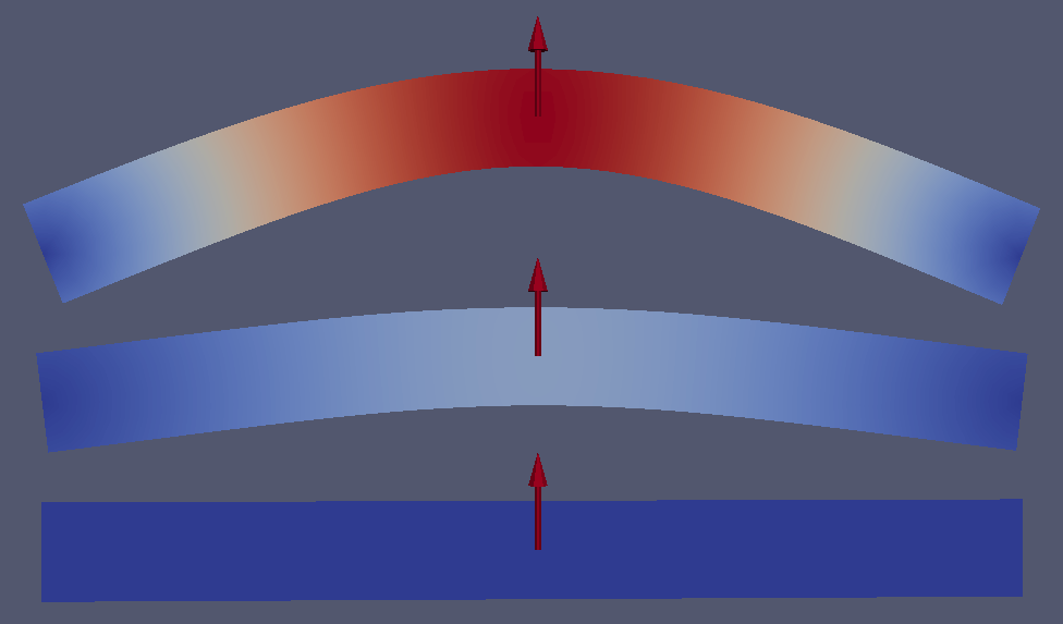
Fig. 33 Deformed beam at three different times (displacement \(\times 10\)).
Static test cases (2D)
- Sources:
- Location:
examples/c++/solid_mechanics_model/static
In static, an example of how to solve a static problem is presented. The
problem geometry is shown in Fig. 34. The left and bottom side
of a 2D plate are blocked with rollers and nodes from the left side are
displaced upward by \(0.01\%\) of the length of the plate.

Fig. 34 Boundary conditions for the static example.
The solution for the static analysis is shown in Fig. 35.
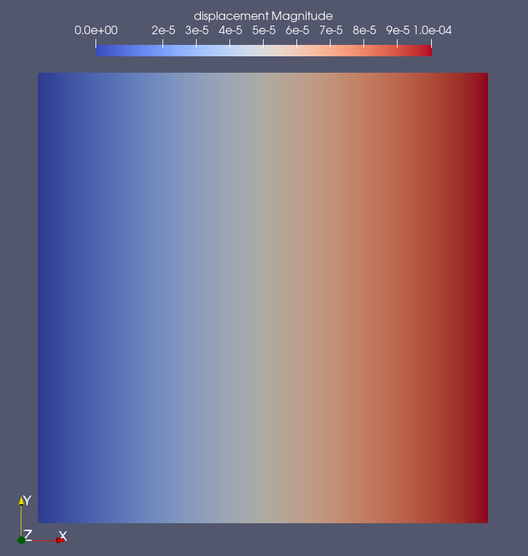
Fig. 35 Solution of the static analysis: displacement magnitude.
parallel (2D)
- Sources:
- Location:
examples/c++/solid_mechanics_model/parallel
In parallel, an example of how to run a 2D parallel simulation is presented.
First, the mesh needs to be distributed among the processors. This is done with:
const auto & comm = Communicator::getStaticCommunicator();
Int prank = comm.whoAmI();
if (prank == 0) {
    mesh.read("square_2d.msh");
}
mesh.distribute();
Here prank designate the processor rank. The mesh is read only by processor 0 and then distributed among all the processors.
All the prints are done only by processor 0. For instance:
if (prank == 0) {
    std::cout << model.getMaterial(0) << std::endl;
}
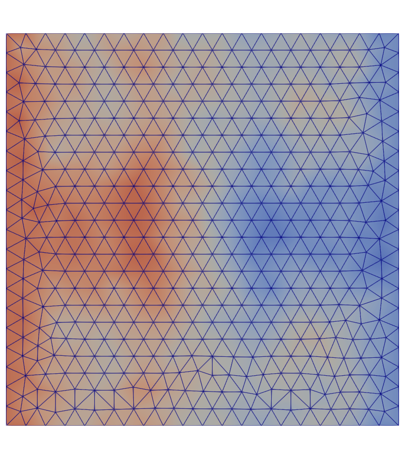
Fig. 36 Displacement in the x direction.
Boundary conditions usage (2D)
- Sources:
- Location:
examples/c++/solid_mechanics_model/boundary_conditions
In predefined_bc it is shown how to impose Dirichlet boundary condition
using the predefined BC::Dirichlet::FixedValue
(Fig. 37). Three built-in Dirichlet functors exist:
FixedValue, FlagOnly and IncrementValue.

Fig. 37 Dirichlet boundary conditions for the predifined_bc case.
To define another functor, a class inherited from
BC::Dirichlet::DirichletFunctor can be created as illustrated in the example
user_defined_bc where a sinusoidal BC is imposed. The corresponding
sinusoidal displacement is depicted in Fig. 38. Note
that a Neumann BC is also imposed.
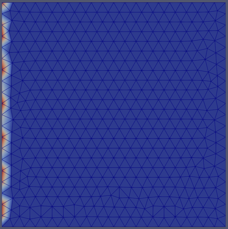
Fig. 38 Displacement magnitude for the user_defined_bc example.
new_material (2D)
- Sources:
- Location:
examples/c++/solid_mechanics_model/new_material
In new_material it is shown how to use a user-defined material for the simulation. All the details are described in Adding a New Constitutive Law. The geometry solved is shown in Fig. 39.

Fig. 39 Problem geometry.
parser (2D)
- Sources:
- Location:
examples/c++/solid_mechanics_model/io/parser
In io/parser, an example illustrating how to parse an input file with user-defined parameters is shown. As before, the text input file of the simulation is precised using the method initialize. In the input file, additionally to the usual material elastic section, there is a section user parameters with extra user-defined parameters.
Within the main function, those parameters are retrived with:
const ParserSection & usersect = getUserParser();
Real parameter_name = usersect.getParameter("parameter_name");
dumper (2D)
- Sources:
- Location:
examples/c++/solid_mechanics_model/io/dumper
In io/dumper, examples of advanced dumping are shown.
dumper_low_level aims at illustrating how to manipulate low-level methods of DumperIOHelper. The goal is to visualize a colorized moving train with Paraview.
It is shown how to dump only a part of the mesh (here the wheels) using the function createElementGroup of the mesh object:
ElementGroup & wheels_elements = mesh.createElementGroup("wheels", spatial_dimension);
One can then add an element to the group with:
wheels_elements.append(mesh.getElementGroup("lwheel_1"));
where lwheel_1 is the name of the element group in the mesh.
Fig. 40 The wheels and the full train are dumped separately.
dumpable_interface does the same as dumper_low_level but using dumpers::Dumpable which is an interface for other classes (Model, Mesh, …) to dump themselves.
Solid Mechanics Cohesive Model
Solid mechanics cohesive model examples are shown in solid_mechanics_cohesive_model. This new model is called in a very similar way as the solid mechanics model:
SolidMechanicsModelCohesive model(mesh);
Cohesive elements can be inserted intrinsically (when the mesh is generated) or extrinsically (during the simulation).
cohesive_intrinsic (2D)
- Sources:
- Location:
examples/c++/solid_mechanics_cohesive_model/cohesive_intrinsic
In cohesive_intrinsic, an example of intrinsic cohesive elements is shown.
An intrinsic simulation is initialized by setting the _is_extrinsic argument of model.initFull to false:
model.initFull(_analysis_method = _explicit_lumped_mass, _is_extrinsic = false);
The cohesive elements are inserted between \(x = -0.26\) and \(x =
-0.24\) before the start of the simulation with
model.getElementInserter().setLimit(_x, -0.26, -0.24);. Elements to the
right of this limit are moved to the right. The resulting displacement is shown
in Fig. 41.
With intrinsic cohesive elements, a bi-linear or exponential cohesive law should
be used instead of a linear one (see section
Intrinsic approach). This is set in the file material.dat:
material cohesive_bilinear [
     name = cohesive
     sigma_c = 1
     beta = 1.5
     G_c = 1
     delta_0 = 0.1
     penalty = 1e10
]
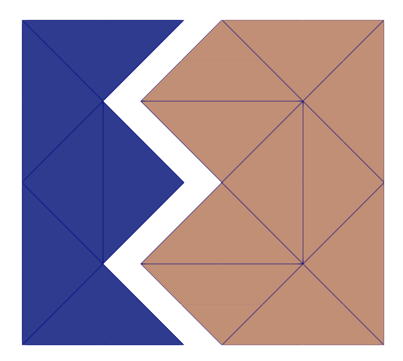
Fig. 41 Displacement in the x direction for the cohesive_intrinsic example.
cohesive_extrinsic (2D)
- Sources:
- Location:
examples/c++/solid_mechanics_cohesive_model/cohesive_extrinsic
In cohesive_extrinsic, an example of extrinsic cohesive elements is shown.
An extrinsic simulation is initialized by setting _is_extrinsic argument of model.initFull to true:
model.initFull(_analysis_method = _explicit_lumped_mass, _is_extrinsic = true);
Cohesive elements are inserted during the simulation but at a location restricted with:
CohesiveElementInserter & inserter = model.getElementInserter();
inserter.setLimit(_y, 0.30, 0.20);
model.updateAutomaticInsertion();
During the simulation, stress has to be checked in order to insert cohesive elements where the stress criterion is reached. This check is performed by calling the method checkCohesiveStress before each step resolution:
model.checkCohesiveStress();
model.solveStep();
For this specific example, a displacement is imposed based on the elements location. The corresponding displacements is shown in Fig. 42.

Fig. 42 Displacement in the y direction for the cohesive_extrinsic example.
cohesive_extrinsic_ig_tg (2D)
- Sources:
- Location:
examples/c++/solid_mechanics_cohesive_model/cohesive_extrinsic_ig_tg
In cohesive_extrinsic_ig_tg, the insertion of cohesive element is not
limited to a given location. Rather, elements at the boundaries of the block and
those on the inside have a different critical stress sigma_c. This is done
by defining two different materials in the examples/c++/solid_mechanics_cohesive_model/cohesive_extrinsic_ig_tg/material.dat.
In this case the cohesive materials are chosen based on the bulk element on both
side. This is achieved by defining MaterialCohesiveRules
The four block sides are then moved outwards. The resulting displacement is shown in Fig. 43.
Fig. 43 Displacement magnitude for the cohesive_extrinsic_ig_tg example.
Contact Mechanics Model
Hertzian contact (2D)
- Sources:
- Location:
examples/c++/contact_mechanics_model/hertz
contact_explicit_static and contact_explicit_dynamic are solving a 2D Hertz contact patch test using the CouplerSolidContact.
The two examples follow what is described extensively in section Coupling with SolidMechanicsModel. The only main difference between contact_explicit_static and contact_explicit_dynamic is the solver used:
// for contact_explicit_static
coupler.initFull(_analysis_method = _static);
// for contact_explicit_dynamic
coupler.initFull(_analysis_method = _explicit_lumped_mass);
The material.dat file contain a contact_detector and a contact_resolution penalty_linear section as explains in section Contact detection.

Friction (2D)
- Sources:
- Location:
examples/c++/contact_mechanics_model/friction
In bloc_friction.cc, a simple example of 2D friction is presented, using the Contact Mechanics model in a dynamic situation.
A block is compressed against a wall, before undergoing a constrained lateral displacement from its upper surface.
A friction coefficient of 0.3 is imposed at the interface, creating a stick-and-slip phenomenon.
The material and contact parameters are set up in the material.dat file.
The wall and the block, lower and upper respectively, have the same properties.
The contact_detector is used to define the numerical parameters for calculating the contact.
Finally, contact_resolution is used for the interface properties, and the penalties to be applied for numerical resolution.
Here, a linear penalty is applied.
mu defines the coefficient of friction, and can be freely modified.
epsilon represents numerical penalties to be applied in order to maintain contact at the interface, and must be set by the user during the simulation.
epsilon_n is used to prevent the two interfaces from interpenetrating, and epsilon_t to detect friction.
is_master_deformable is set to false to ignore wall deformation, in order to reduce calculation times.

Fig. 44 Friction of a bloc against a wall with mu = 0.3.
Diffusion Model (2D and 3D)
- Sources:
- Location:
examples/c++/diffusion_model
In diffusion_model, examples of the HeatTransferModel are presented.
An example of a static heat propagation is presented in
heat_diffusion_static_2d.cc. This example consists of a square 2D plate of
\(1 \text{m}^2\) having an initial temperature of \(100 \text{K}\)
everywhere but a non centered hot point maintained at
\(300 \text{K}\). Fig. 45 presents the geometry
of this case (left) and the results (right). The material used is a linear
fictitious elastic material with a density of \(8940 \text{kg}/\text{m}^3\),
a conductivity of \(401 \text{W}/\text{m}/\text{K}\) and a specific heat
capacity of \(385 \text{J}/\text{K}/\text{kg}\).
The simulation is set following the procedure described in Using the Heat Transfer Model
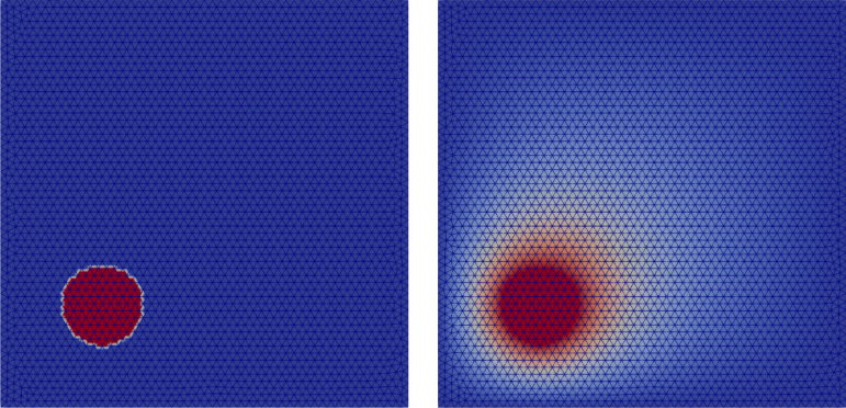
Fig. 45 Initial (left) and final (right) temperature field
- Sources:
In heat_diffusion_dynamics_2d.cc, the same example is solved dynamically
using an explicit time scheme. The time step used is \(0.12 \text{s}\). The only main difference with the previous example lies in the model initiation:
model.initFull(_analysis_method = _explicit_lumped_mass);

Fig. 46 Temperature field after 15000 time steps = 30 minutes. The lines represent iso-surfaces.
- Sources:
In heat_diffusion_dynamics_3d.cc, a 3D explicit dynamic heat propagation
problem is solved. It consists of a cube having an initial temperature of
\(100 \text{K}\) everywhere but a centered sphere maintained at
\(300 \text{K}\).
The simulation is set exactly as heat_diffusion_dynamics_2d.cc except that the mesh is now a 3D mesh and that the heat source has a third coordinate and is placed at the cube center.
The mesh is initialized with:
Int spatial_dimension = 3;
Mesh mesh(spatial_dimension);
mesh.read("cube.msh");
Fig. 47 presents the resulting temperature field evolution.

Fig. 47 Temperature field evolution.
Phase-field model (2D) [Unstable]
static
- Sources:
- Location:
examples/c++/phase_field_model
phase_field_notch.cc shows hot to set a quasi-static fracture simulation with phase-field. The geometry of the solid is a square plate with a notch. The loading is an imposed displacement at the top of the plate (mode I).

Fig. 48 Notched plate with boundary conditions and imposed displacement.
In addition, this example shows how to extract clusters delimited by the mesh boundaries and elements with damage values beyond a threshold. This can be useful to extract fragments after crack propagation.
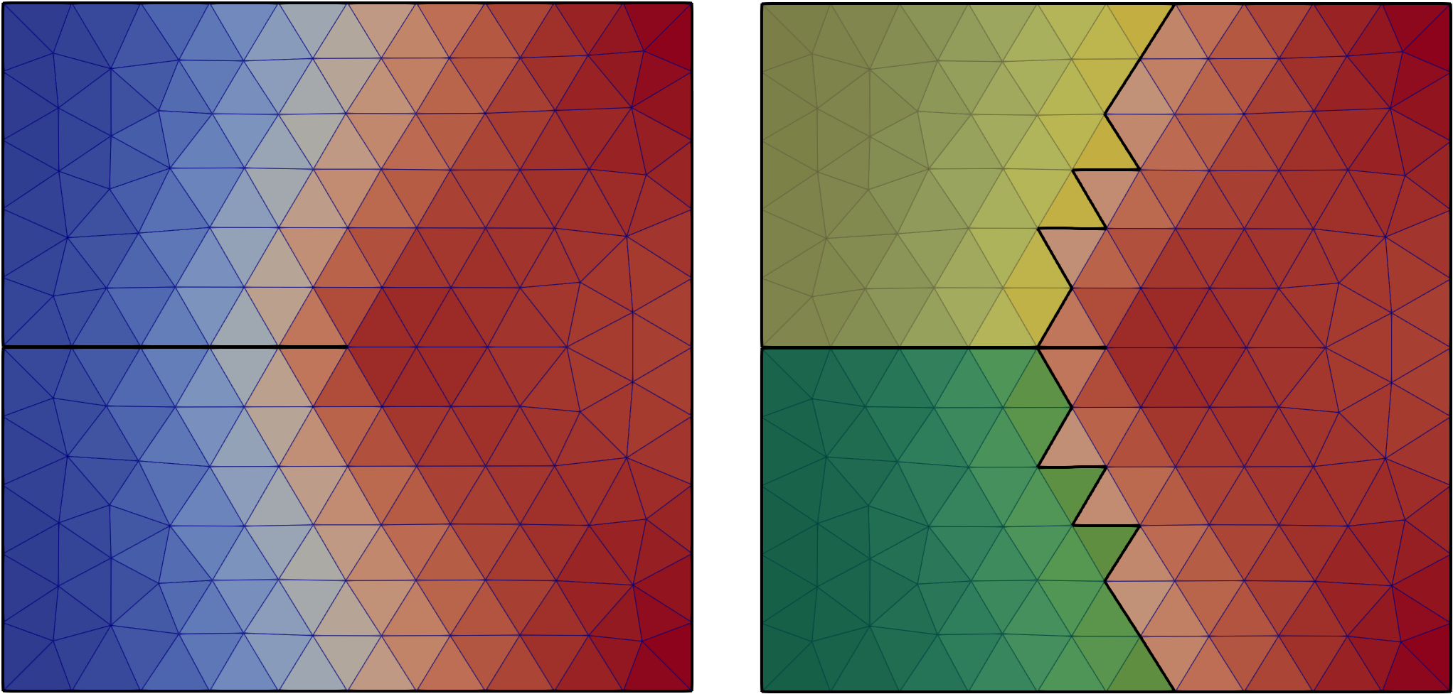
Fig. 49 Damage field after a few iterations and two clusters (fragments) extracted.
Scalability test (3D)
- Sources:
- Location:
examples/c++/scalability_testThis example is used to do scalability test, with elastic material or cohesive elements inserted on the fly. The cube.geo should generate a mesh with roughly 4’500’000 elements and 730’000 nodes. The cube.msh file included is a tiny cube only to test if the code works.
To run the full simulation the full mesh has to be generated gmsh -3 cube.geo -o cube.msh
The simulation consist of a cube with a compressive force on top and a shear force on four sides as shown in the figure bellow

This examples was used to run the scalability test from the JOSS paper the full mesh and results presented in the following graph can be found here: perf-test-akantu-cohesive

Python examples
To run simulations in Python using Akantu, you first need to import the module:
import akantu as aka
The functions in Python are mostly the same as in C++.
The initiation differs. While in C++ a function is initialized using initialize("material.dat", argc, argv);, in Python you should do:
aka.parseInput('material.dat')
The creation and loading of the mesh is done with:
mesh = aka.Mesh(spatial_dimension)
mesh.read('mesh.msh')
Solid Mechanics Model
The Solid Mechanics Model is initialized with:
model = aka.SolidMechanicsModel(mesh)
plate_hole (2D)
- Sources:
- Location:
examples/python/solid_mechanics_model/plate-hole
In plate_hole, an example of a static solution of a loaded plate with a hole. Because of the symmetries, only a quarter of the problem is modeled. The corresponding domain and boundary conditions is shown in Fig. 50.
The static solver is initialized with:
model.initFull(_analysis_method=aka._static)
Boundary conditions are applied with:
model.applyBC(aka.FixedValue(0.0, aka._x), "XBlocked")
model.applyBC(aka.FixedValue(0.0, aka._y), "YBlocked")
model.applyBC(aka.FromTraction(trac), "Traction")
where trac is a numpy array of size spatial_dimension.
Additionally, the simulation can be run in parallel. To do so, the following lines are added:
try:
  from mpi4py import MPI
  comm = MPI.COMM_WORLD
  prank = comm.Get_rank()
except ImportError:
  prank = 0
Similarly to C++, the mesh has to be distributed between the processors with:
mesh.distribute()

Fig. 50 Plate with a hole geometry.
The displacement magnitude is displayed in Fig. 51.
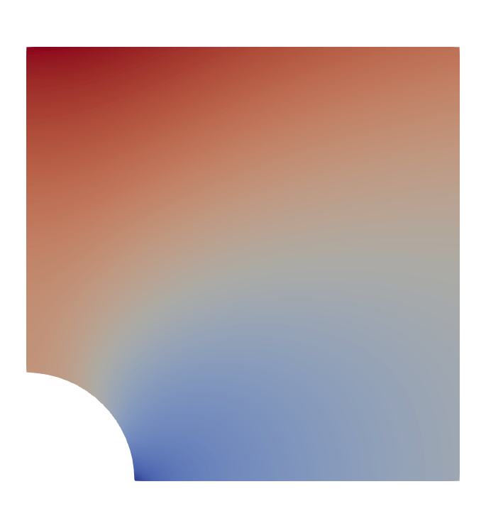
Fig. 51 Displacement magnitude.
dynamics (2D)
- Sources:
- Location:
examples/python/solid_mechanics_model/dynamics
In dynamics, an example of a dynamic simulation solved with an explicit time intergration is shown. This examples
model the propagation of a wave in a bar. The geometry is depicted in Fig. 52. A pulse is impose
as an initial displacement over the bar. Results are depicted in Fig. 53.
The explicit time integration scheme is set with:
model.initFull(_analysis_method=aka._explicit_lumped_mass)
This example shows how to create a new functor to set the boundary conditions. This is done by creating a class that inherits from aka.FixedValue (MyFixedValue(aka.FixedValue) in this case).
The boundary conditions are then applied with:
model.applyBC(MyFixedValue(0, aka._x), "XBlocked")
model.applyBC(MyFixedValue(0, aka._y), "YBlocked")

Fig. 52 Plate with a hole geometry.

Fig. 53 Displacement magnitude.
eigen_modes (2D)
- Sources:
- Location:
examples/python/solid_mechanics_model/eigen_modes
In eigen_modes it is shown how to compute the eigen modes using the library scipy.sparse. The mode can be specify with the -m argument. Simulation is performed on a bar where a pulse is imposed.
The -p argument will plot the following figures Fig. 54:
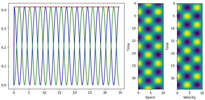
Fig. 54 Energy norms as a fonction of time (left), space-time diagram for diplacements (center) and space-time diagram for velocities (right) with the default values.
- An implicit time integration scheme is used and set with::
model.initFull(aka._implicit_dynamic)
custom-material (2D)
- Sources:
- Location:
examples/python/solid_mechanics_model/custom-material
In custom-material.py it is shown how to create a custom material behaviour. In this example, a linear elastic
material is recreated. It is done by creating a class that inherits from aka.Material (LocalElastic(aka.Material) in this case) and register it
to MaterialFactory:
class LocalElastic(aka.Material):
    [...]

def allocator(_dim, unused, model, _id):
    return LocalElastic(model, _id)

mat_factory = aka.MaterialFactory.getInstance()
mat_factory.registerAllocator("local_elastic", allocator)
Wave propagation of a pulse in a bar fixed on the top, bottom and right boundaries is simulated using an explicit scheme. Results are shown in Fig. 55.

Fig. 55 Wave propagation in a bar.
In bi-material.py, the same principle is used to create a bimaterial square. The displacement is shown in Fig. 56.
In this example a simpler way but less versatile way of registering the custom material is demonstrated:
class LocalElastic(aka.Material):
    [...]

aka.registerCustomMaterials({"local_elastic": LocalElastic})
In this example the parseInput is also replaced by the material parameters given to the initFull function:
model.initFull({"fictive": {
  "type": "local_elastic",
  "rho": 1.,
  "E": 1.,
  "nu": .3}}, _analysis_method=aka._static)
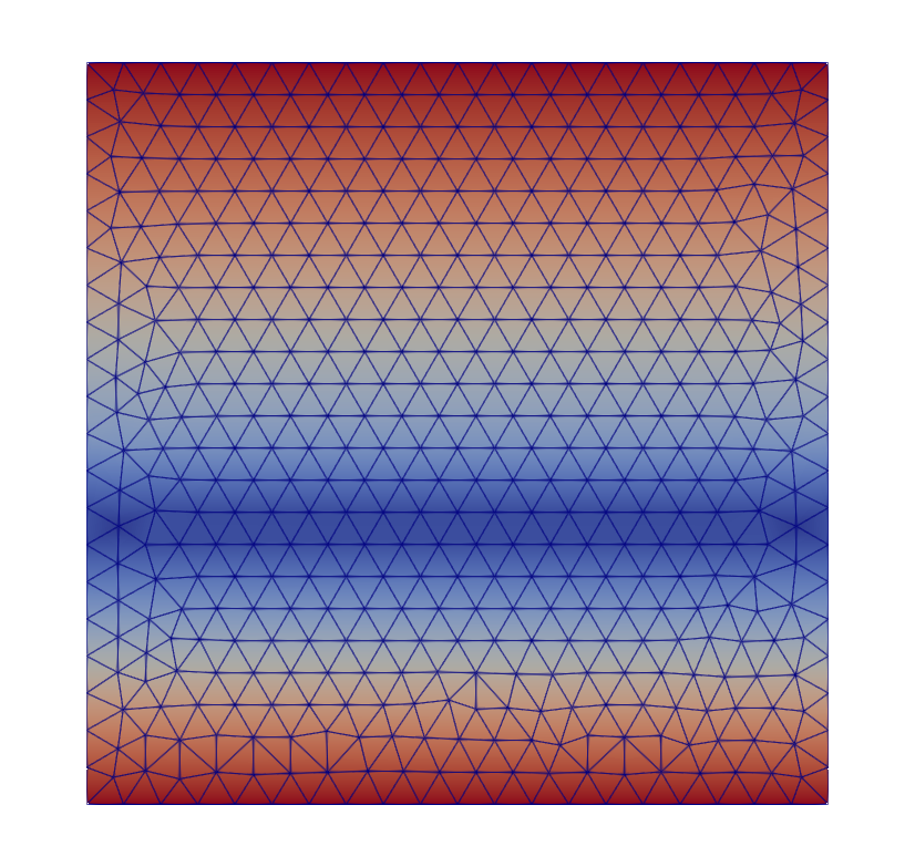
Fig. 56 Bimaterial square.
stiffness_matrix (2D)
- Sources:
- Location:
examples/python/solid_mechanics_model/stiffness_matrix
stiffness_matrixshows how to get the stiffness matrix from a mesh. It is done with::model.assembleStiffnessMatrix() K = model.getDOFManager().getMatrix(‘K’) stiff = aka.AkantuSparseMatrix(K).toarray()
solver_callback (2D)
- Sources:
- Location:
examples/python/solid_mechanics_model/solver_callback
In solver_callback, it is shown how to write a solver callback function. It is done by writing a class that inherit
from InterceptSolverCallback:
class SolverCallback(aka.InterceptSolverCallback):
        [.....]

solver_callback = SolverCallback(model)

model.solveStep(solver_callback)
In that case, the solver callback is used to modify the stiffness matrix.
Solid Mechanics Cohesive Model
cohesive (2D)
- Sources:
- Location:
examples/python/solid_mechanics_cohesive_model/cohesive
In cohesive/plate.py, an example of extrinsic cohesive elements insertion is shown. This example simulates a plate
with a pre-existing crack pulled. The geometry is depicted in Fig. 57.

Fig. 57 Problem geometry.
The problem is solved statically until the onset of instability and is then solved dynamically with an explicit
integration scheme. This is done by adding a new solver with model.initNewSolver():
model = aka.SolidMechanicsModelCohesive(mesh)
model.initFull(_analysis_method=aka._static, _is_extrinsic=True)
model.initNewSolver(aka._explicit_lumped_mass)
[....]
model.solveStep("static")
[....]
model.solveStep("explicit_lumped")
The crack opening is displayed in Fig. 58.
Fig. 58 Stresses in the plate.
fragmentation (2D)
- Sources:
- Location:
examples/python/solid_mechanics_cohesive_model/fragmentation
fragmentation shows an example of a 1D bar fragmentation with extrinsic cohesive elements. It uses a custom boundary
condition to impose a constant velocity. This is done by creating a class that inherits from DirichletFunctor.
The result is shown in Fig. 59.

Fig. 59 1D bar fragmentation.
multi-material (2D)
- Sources:
- Location:
examples/python/solid_mechanics_cohesive_model/multi-material
This example is the same as example as the Sources example The main difference is that in this example there are multiple cohesive laws. The way they are selected is by using a aka.MaterialCohesiveRulesSelector
cohesive_selector = aka.MaterialCohesiveRulesSelector(model, {
  ("Top", "Bottom"): "tough",
  ("Top", "Top"): "soft",
  ("Bottom", "Bottom"): "soft",
})

model.setMaterialSelector(cohesive_selector)
Contact Mechanics Model
Compression (2D)
- Sources:
- Location:
examples/python/contact_mechanics_model/compression
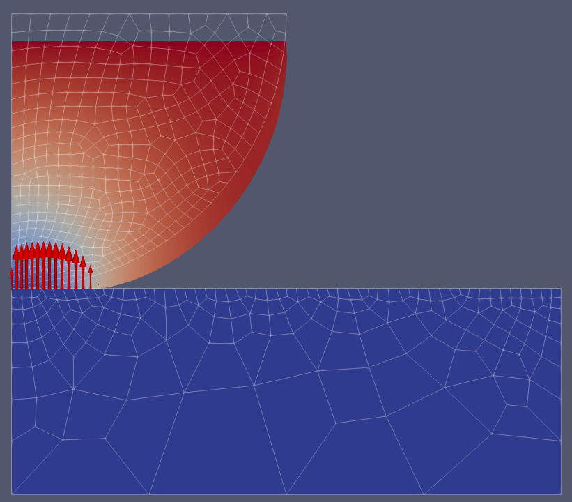
In compression.py it is shown how to couple the Solid Mechanics Model with the Contact Mechanics Model. The example simulate the contact betweem two blocks.

Friction (2D)
- Sources:
- Location:
examples/python/contact_mechanics_model/friction
In friction.py it is shown how to couple the Solid Mechanics Model with the Contact Mechanics Model, applying the friction law. The example simulate the contact between two blocks with a friction coefficient of 0.3. It is similar to the ‘bloc_friction.cc’ example in C++.
Fig. 60 Friction of a bloc against a wall with mu = 0.3.
Phase-field model (2D)
static
- Sources:
- Location:
examples/python/phase_field_model
phasefield-static.py shows how to setup a static phase-field fracture simulation. An imposed displacement is imposed on the top of a notched square plate.
Fig. 61 Notched plate with boundary conditions and imposed displacement.
In static simulations, we use loading steps to apply the displacement incrementally. At each time step, the solvers of the solid mechanics model and the phase-field model are called alternately until convergence is reached.
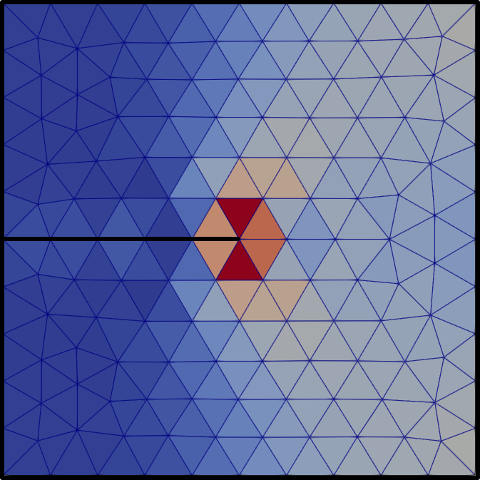
Fig. 62 Damage field after a few iterations.
dynamic
- Sources:
phasefield-dynamic.py shows how to setup a dynamic phase-field fracture simulation. A notched plate is pre-strained in mode I using Dirichlet BC and a static solve. The simulation is then continued in dynamic using an explicit Neumark scheme.

Fig. 63 Notched plate with boundary conditions and imposed displacement.
At each time step, each solver is called once to find the displacement field and the damage field.
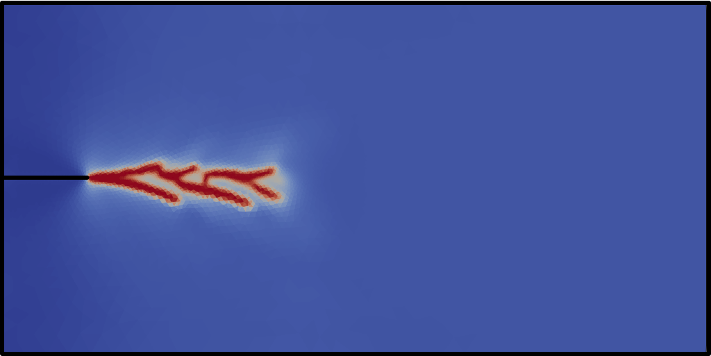
Fig. 64 Crack propagation and branching.