PhaseField Model

The phasefield model is a specific implementation of Model interface to handle brittle fracture for infinitesimal strains.

Theory

The variational formulation of brittle fracture was first proposed by Francfort and Marigo:cite:franc so as to overcome the shortcomings of Griffith’s criteria. The approach used by Francfort and Margio for variational formulation is based on the principle of global minimality of total energy. Similar to Griffith’s work, they define a surface energy corresponding to the discontinuity \(\Gamma\) as

\[\Phi_{s}(\Gamma) = \int\limits_{\Gamma}\mathcal{G}_cd\mathcal{H}^{d-1}(\Gamma)\]

where \(\mathcal{H}^{d-1}\) is d-1 dimensional Hausdroff measure which is surface measure for smooth hypersurfaces. the material behavior is considered to be linearly elastic with small strains throughout the body. Based on these assumptions the elastic energy of the body is defined as

\[\Phi_e(\Gamma,u) = \int\limits_{\Omega_{p}}\psi(\boldsymbol{\epsilon}(u))d\Omega\]

where \(\psi\) is elastic energy density and it is given as a function of strain as

\[\psi_e(\boldsymbol{\epsilon}) = \dfrac{1}{2}\lambda(\text{tr}(\boldsymbol{\epsilon}))^{2}+\mu\boldsymbol{\epsilon}:\boldsymbol{\epsilon}\]

Exponential phasefield law

Bourdin et. al.:cite:bourdin in their work proposed a regularized version of variational formulation where a scalar field variable \(d(\vec{x},t)\) is used to represent crack. This scalar field variable approximates the sharp crack topology by taking value 1 at crack location and smoothly diffusing into value 0 away from the crack. figref{fig:diffusive_topology} shows both sharp crack topology and an approximated regularized crack topology for one-dimensional case.

The strong form of the phasefield can be expressed as

\[2(1-d)\mathcal{H} - \dfrac{G_c}{l_0}(d-l_0^2d) = 0 \nabla d . \boldsymbol n = 0\]

Using the PhaseField Model

The PhaseFieldModel object solves the strong form using an inplicit solver. An instance of the class can be created like this:

PhaseFieldModel phase(mesh, spatial_dimension);

while ans existing mesh has been used (see ref{sect:common:mesh}). To intialize the model object:

phase.initFull();

Currently, implicit solver is defined for the phasefield model and no explicit solver is implemented in Akantu. Furthermore, By default, the implicit solver defined is of linear type. One can change the linear solver to a non-linear by initiating a new solver type.

The phasefield model contains Arrays:

damage:

contains the nodal damage \(d\) (zero by default after the initialization)

blocked_dofs

contains a Boolean value specifying whether the damage at a node is to be blocked or not. A Dirichlet boundary condition can be prescribed by setting the blocked_dofs value of damage to true. The damage ais computed for all nodes where the blocked_dofs value is set to false. For the remaining nodes, the imposed values (zero by default after initialization) are kept.

internal_force

contains the driving force responsible for the crack to nucelate or propagate.

Currently, the phasefield model uses a exponential shaped scalar field variable \(d(\vec{x}, t)\) to approximate the sharp crack topology. A Phasefield variable thus requires a length scale parameter \(l_0\) to control the width of the diffusive crack topology along with the material parameters such as elastic modulus, poisson’s ratio, critical energy release rate.

The data input file provides the parameters for the exponential phasefield law as follows:

phasefield exponential [
           name = plate
           E = 210.0
           nu =  0.3
           gc = 5e-3
           l0 = 0.1
]

PhaseFieldModel can handle

phasefield laws for multiple materials. To define so:

phasefield exponential [
           name = hard
           E = 210.0
           nu =  0.3
           gc = 5e-3
           l0 = 0.1
]

phasefield exponential [
           name = soft
           E = 21.0
           nu =  0.3
           gc = 5e-5
           l0 = 0.1
]

In order to assign correct phasefield variable properties based on the names of region as defined in mesh file, MeshDataPhaseFieldSelector must be set as phasefield selector:

auto && selector = std::make_shared<MeshDataPhaseFieldSelector<std::string>>(
        "physical_names", phase);
phase.setPhaseFieldSelector(selector);

For the crack to nucleate or propagate, phasefield model requires strain measure at each quadrature point. The strain measure computed from solid mechanics model is provided to the phasefield model. Similarly, damage value computed at each quadrature point by the phasefield model is provided to the solid mechanics model. This damage is thus used to degrade the the elastic strain energy. To do so, a new material which is a specific implementation of MaterialDamage is defined for solid mechanics model. The governing equation is given as

\[\boldsymbol \sigma = ((1-d)^2 + \eta)\dfrac{\psi}{\boldsymbol \epsilon}\]

where \(\psi\) is the elastic energy and \(\eta\) is a numerical parmaeter avoid numerical difficulties due to full degradation of elastic energy for fully broken state. The material properties are thus provided in the input data filled as:

material phasefield [
      name = hard
      rho = 1.
      E = 210.0
      nu = 0.3
      eta = 0.0
      Plane_Stress = false
]

material phasefield [
      name = soft
      rho = 1.
      E = 21.0
      nu = 0.3
      eta = 0.0
      Plane_Stress = false
]

To simplify the execution of phasefield model coupled with solidmechanis model, a special class CouplerSolidPhaseField is provided.

Coupling Phase Field Model and Solid Mechanics Model

A dedicated coupler class CouplerSolidPhaseField is defined in Akantu to ease the coupling of the two models.

When an instance of a Coupler class is created, it automatically creates the instances of solid mechanics model and phasefield model. The two objects can be retrived from the coupler class.

CouplerSolidPhaseField coupler(mesh);
auto & phase = coupler.getPhaseFieldModel();
auto & solid = coupler.getSolidMechanicsModel();

The two objects must be used to define the solver type and apply boundary conditions.

solid.initFull(_analysis_method = _explicit_lumped_mass);
phase.initFull(_analysis_method = _static);

The whole process of coupling the two models at a given time step is made easy by the solve function of coupler class.

coupler.solve(<solver_id_for_solid_model>, <solver_id_for_phasefield_model>);

Staggered scheme

To solve the solid mechanics model and phasefield model, staggered scheme is implemented. In staggered scheme, at current time step first solid mechanics model is solved assuming the damage values from the previous time step. The strain thus computed are passed to the phasefield model and now, phasefield model is solved for the damage variable. At each iteration step, convergence in displacement and damage is checked for. If convergence is not reached, the combined newton-raphson iteration continues.

To illustrate the staggered scheme solution of phasefield model, one can refere to the examples provided for the phasefield model. Two examples provided are for static phasefield-static.py and dynamic crack propgation phasefield-dynamic.py.

For the static problem, both the solid mechanics model and the phsefield model are solved using alinear implicit solver. Convergence in value of both displacement as well as damage is checked at each loading step.

In case of the dynamic problem, solid mechanics model is solved dynamically using an explicit solver and the phasefield model is solved using a linear implcit solver. In this sceanrio, the staggered scheme doesnot check for any convergence. Below is the crack propagation observed for the dyanmic problem.

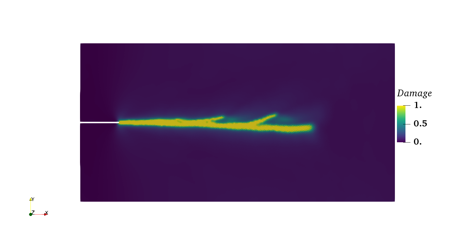
Dynamic crack propagation using phasefield model